Note from Towards Data Science’s editors: While we allow independent authors to publish articles in accordance with our rules and guidelines, we do not endorse each author’s contribution. You should not rely on an author’s works without seeking professional advice. See our Reader Terms for details.

Towards Data Science编辑的注意事项： 尽管我们允许独立作者按照我们的 规则和指南 发表文章 ，但我们不认可每位作者的贡献。 您不应在未征求专业意见的情况下依赖作者的作品。 有关 详细信息， 请参见我们的 阅读器条款 。

A common problem when evaluating a portfolio manager is that the history of returns is often so short that estimates of risk and performance measures can be highly unreliable. A similar problem occurs when testing a new trading strategy. Even if you have a fairly long history for the strategy’s performance, often you only have observations over a single market cycle which can make it difficult to evaluate how your strategy would have held up in other markets. If you trade stocks you have probably heard the refrain: “I’ve never seen a bad back test”.

在评估投资组合经理时，一个常见的问题是收益的历史通常很短，以至于风险和绩效指标的估计可能非常不可靠。 测试新的交易策略时会发生类似的问题。 即使您对策略的执行历史已有很长的历史，但通常您只能在单个市场周期中观察到，这可能使您难以评估您的策略在其他市场中的表现。 如果您交易股票，您可能会听到这样的话：“我从未见过糟糕的回测”。

One method to address this deficiency is through Factor Model Monte Carlo (FMMC). FMMC can be used to estimate a factor model based on a set of financial and economic factors that reliably explain the returns of the fund manager. We can then simulate returns to determine how the manager would have performed in a wide variety of market environments. The end result is a model that produces considerably better estimates for risk and performance than if we simply used the return series available to us.

解决此缺陷的一种方法是通过因素模型蒙特卡洛(FMMC) 。 FMMC可用于基于一组可靠地解释基金经理收益的财务和经济因素来估计因素模型。 然后，我们可以模拟收益，以确定经理在各种市场环境中的表现。 最终结果是，与仅使用可用的收益序列相比，该模型可以更好地估算风险和绩效。

任务和设置 (The Task and Set Up)

For this case study, we will be analyzing the returns for the new hedge fund Aric’s Hedge Fund; hereafter known as AHF. The hedge fund case is particularly interesting because hedge funds can use leverage, invest in any asset class, go long or short, and use many different instruments. Hedge funds are often very secretive about their strategy and holdings. Thus, having a reliable risk model to explain the source of their returns is essential.

在本案例研究中，我们将分析新对冲基金Aric's Hedge Fund的回报； 以下简称AHF 。 对冲基金的案例特别有趣，因为对冲基金可以利用杠杆，投资于任何资产类别，做多或做空以及使用许多不同的工具。 对冲基金通常对其策略和持股非常保密。 因此，拥有可靠的风险模型来解释其收益的来源至关重要。

Keep in mind that Aric’s Hedge Fund is not a real hedge fund (I’m Aric, I don’t have a hedge fund), but this is a real series of returns. I obtained the returns for a hedge fund in operation that we invest in where I work so the results of this study are applicable to a real-world scenario.

请记住，Aric的对冲基金不是真正的对冲基金(我是Aric，我没有对冲基金)， 但这是一系列真实的回报。 我获得了对冲基金的回报，该对冲基金投资于我工作的地方，因此本研究的结果适用于现实情况。

We have data for Aric’s Hedge Fund from January 2010 to March 2020. For the purpose of this post and evaluating the accuracy of our model we will pretend as though AHF is pretty new to the scene and that we only have data from January 2017 through March 2020. To overcome the data deficiency, we will build a factor model on the basis of this “observed data” and then utilize the entire data series to evaluate the accuracy of our simulation for assessing the risk and performance statistics.

我们拥有2010年1月至2020年3月Aric对冲基金的数据。出于这篇文章的目的，并评估我们模型的准确性，我们将假装 AHF尚不成熟，并且我们仅提供2017年1月至3月的数据。 2020年。为克服数据不足，我们将在此“观察数据”的基础上建立一个因子模型，然后利用整个数据系列来评估模拟的准确性，以评估风险和绩效统计数据。

The below graph shows the cumulative return of AHF since January 2010. The data to the right of the red line represents the “observed period”.

下图显示了自2010年1月以来AHF的累计收益。红线右侧的数据代表“观察期”。

We will be conducting the analysis in R using the extensive library of packages available therein including: PerformanceAnalytics and quantmod. Aside from the hedge fund returns series, all of the factor data can be obtained freely from Yahoo! Finance, the Federal Reserve Bank of St. Louis FRED Database, and the Credit Suisse Hedge Fund Indices; you have to sign up for Credit Suisse to access the indices, but still…free.

我们将使用其中提供的广泛的软件包库在R中进行分析，包括： PerformanceAnalytics和quantmod 。 除了对冲基金收益系列以外，所有因子数据都可以从Yahoo!免费获得。 金融 ，圣路易斯联邦储备银行FRED数据库和瑞士信贷对冲基金指数 ； 您必须注册瑞士信贷才能访问该指数，但仍然…免费。

模型估计 (Model Estimation)

A common technique in empirical finance is to explain changes in asset prices based on a set of common risk factors. The simplest and most well-known factor model is the Capital Asset Pricing Model (CAPM) of William Sharpe. The CAPM is specified as follows:

经验金融中的一种常见技术是基于一组常见风险因素来解释资产价格的变化。 最简单和最著名的因素模型是William Sharpe的资本资产定价模型(CAPM)。 CAPM指定如下：

Where:

哪里：

• ri = Return of asset ‘i’ri =资产“ i”的收益
• m = Return of market index ‘m’m =市场指数“ m”的回报
• ∝= Excess return∝ =超额收益
• ẞ = Exposure to the Market Risk factorẞ=暴露于市场风险因素
• Ɛi = Idiosyncratic error term= i =特异误差项

Market risk, or “systematic” risk, serves as a summary measure for all of the risks to which financial assets are exposed. This may include recessions, inflation, changes in interest rates, political turmoil, natural disasters, etc. Market risk is usually proxied by the returns on a large index like the S&P 500 and cannot be reduced through diversification.

市场风险或“系统性”风险，是金融资产​​所面临的所有风险的汇总度量。 这可能包括衰退，通货膨胀，利率变化，政治动荡，自然灾害等。市场风险通常由标普500指数等大型指数的回报所替代，并且无法通过多元化降低。

ẞ (i.e. Beta) represents an asset’s exposure to market risk. A Beta = 1 would imply that the asset is as risky as the market, Beta >1 would imply more risk than the market, while a Beta < 1 would imply less risk.

ẞ(即Beta)代表资产的市场风险。 Beta = 1表示资产的风险与市场一样，Beta> 1的风险比市场高，而Beta <1的风险比市场低。

Ɛ is idiosyncratic risk and represents the portion of the return that cannot be explained by the Market Risk factor.

Ɛ是特质风险，代表不能由市场风险因素解释的收益部分。

We will extend the CAPM to include additional risk factors which the literature have shown to be important for explaining asset returns. Aric’s Hedge Fund runs a complicated strategy using many different asset classes and instruments so it’s certainly plausible that it would be exposed to a broader set of risks beyond the traditional market index. The general form of our factor model is as follows:

我们将把CAPM扩展到包括其他风险因素，这些因素已被文献证明对于解释资产收益很重要。 Aric的对冲基金使用许多不同的资产类别和工具来执行一项复杂的策略，因此，它可能会面临比传统市场指数更广泛的风险。 我们的因子模型的一般形式如下：

All the above says is that returns (r) are explained by a set of risk factors j=1…k where r j is the return for factor ‘j’ and ẞ j is the exposure. Ɛ is the idiosyncratic error. Thus, if we can estimate the ẞ j, then we can leverage the long history of factor returns (r j) calculate conditional returns for AHF. Finally, if we can reasonably estimate the distribution of Ɛ then we can build randomness into AHF’s return series. This enables us to fully capture the variety of returns that we could observe.

上面所说的全部是，回报(r)由一组风险因子j = 1…k解释，其中rj是因子“ j”的回报，而ẞj是风险敞口。 Ɛ是特质错误。 因此，如果我们可以估计ẞj，那么我们就可以利用长期的要素收益率(rj)计算AHF的条件收益率。 最后，如果我们可以合理估计distribution的分布，则可以将随机性构建到AHF的收益序列中。 这使我们能够充分捕捉我们可以观察到的各种回报。

The FMMC method will take place in three parts:

FMMC方法将分为三个部分：

• Part A: Data Acquisition, Clean Up and ProcessingA部分：数据采集，清理和处理
• Part B: Model EstimationB部分：模型估算
• Part C: Monte Carlo SimulationC部分：蒙特卡洛模拟

A部分：数据采集，清理和处理 (Part A: Data Acquisition, Clean Up and Processing)

For the factor model I will be using a set of financial and economic variables aimed at measuring different sources of risk and return. Again, all the data used in this study are freely available from Yahoo! Finance, the FRED Database, and Credit Suisse.

对于因子模型，我将使用一组金融和经济变量，旨在衡量风险和回报的不同来源。 同样，本研究中使用的所有数据均可从Yahoo!免费获得。 金融，FRED数据库和瑞士信贷。

We’ll begin with the FRED data. Next to each variable I have placed the unique identifier that you can query from the database.

我们将从FRED数据开始。 在每个变量旁边，我放置了可以从数据库查询的唯一标识符。

FRED Variables:

FRED变量：

• 5-Year Inflation Expectations, 5-Years Forward. (T5YIFRM)未来5年通胀预期，未来5年。 (T5YIFRM)
• Term Spread: 10-Year minus 3-month Treasury Yield Spread. (T10Y3M)期限利差：10年期减去3个月的美国国债收益率利差。 (T10Y3M)
• Credit spread premium: Moody’s Baa corp bond yield minus 10-year Treasury yield. (BAA10Y)信用利差溢价：穆迪的Baa公司债券收益率减去10年期美国国债收益率。 (BAA10Y)
• 3-month T-bill rate. (DGS3MO)3个月期国库券利率。 (DGS3MO)
• TED Spread: 3-Month LIBOR Minus 3-Month Treasury Yield. (TEDRATE)TED利差：3个月伦敦银行同业拆借利率减去3个月国库券收益率。 (TEDRATE)
• International bond yield: 10-Year government bond yields for Euro Area. (IRLTLT01EZM156N)国际债券收益率：欧元区10年期政府债券收益率。 (IRLTLT01EZM156N)
• Corporate Bond Total Return Index: ICE BofAML Corp bond master total return index; in levels. (BAMLCC0A0CMTRIV)公司债券总收益指数：ICE BofAML Corp债券主总收益指数； 在水平上。 (BAMLCC0A0CMTRIV)
• CBOE Volatility Index (i.e. the VIX). (VIXCLS)CBOE波动率指数(即VIX)。 (VIXCLS)
• CBOE Volatility Index of US 10-Year Treasuries (i.e. the Treasury VIX). (VXTYN)美国10年期美国国债(即美国国债VIX)的CBOE波动率指数。 (VXTYN)

The FRED API leaves something to be desired and does not allow you to pull data in a consistent way. The returns of AHF are monthly so our model will need to be estimated using monthly data. However, FRED retrieves data at the highest available frequency so daily data always comes in as daily. Furthermore, the data is retrieved from the beginning of the series, so you end up getting a lot of NAs. As such, we will need to do a little clean up before we proceed.

FRED API有一些不足之处，并且不允许您以一致的方式提取数据。 AHF的回报是每月的，因此我们的模型需要使用每月的数据进行估算。 但是，FRED会以最高可用频率检索数据，因此每日数据始终以每日形式出现。 此外，数据是从本系列的开始检索的，因此您最终会获得很多NA。 因此，在继续之前，我们需要进行一些清理。

The following segments of R code show loading the identifiers into variables and separate queries to FRED for the daily and monthly data. The daily data is cleaned and converted to a monthly frequency. I’ve tried to comment the code as much as possible so you can see what’s happening.

R代码的以下各节显示将标识符加载到变量中，并分别向FRED查询每日和每月数据。 每日数据将被清理并转换为每月一次。 我尝试了尽可能多地注释代码，以便您可以看到发生了什么。

The FRED data is good to go. The other set of variables that we will need are financial market indices. Growth, Value and Size indices feature prominently in asset pricing models such as the Fama-French 3-Factor Model and I take the same approach here. Returns from financial indices are obtained from the venerable Yahoo! Finance.

FRED数据很好。 我们将需要的另一组变量是金融市场指数。 增长，价值和规模指数在诸如Fama-French 3-Factor Model之类的资产定价模型中具有突出的地位，在此我采用相同的方法。 财务指数的收益来自古老的Yahoo! 金融。

Yahoo! Finance Variables:

雅虎！ 财务变量：

• Value: Russell 1000 Value Index (^RLV)值：罗素1000价值指数(^ RLV)
• Growth: Russell 1000 Growth Index (^RLG)成长：罗素1000成长指数(^ RLG)
• Size: Russell 2000 Index (^RUT)大小：罗素2000指数(^ RUT)
• Market: S&P 500 Index (^GSPC)市场：标普500指数(^ GSPC)
• International: MSCI EAFE (EFA)国际：MSCI EAFE(EFA)
• Bonds: Barclays Aggregate Bond Index (AGG)债券：巴克莱综合债券指数(AGG)

Lastly, we’ll load in the hedge fund specific indices courtesy of Credit Suisse (CS). Obtaining the index requires a few extra steps as the data needs to manually downloaded to Excel from the Credit Suisse website and then loaded into R. Each index corresponds to a specific hedge fund strategy.

最后，我们将根据瑞士信贷(CS)的数据加载对冲基金的特定指数。 获取索引需要一些额外的步骤，因为需要将数据从瑞士信贷网站手动下载到Excel，然后加载到R中。每个索引对应于特定的对冲基金策略。

Credit Suisse Variables:

瑞士信贷变量：

• Convertible Bond Arbitrage Index (CV_ARB)可转换债券套利指数(CV_ARB)
• Emerging and Frontier Markets Index (EM_MRKT)新兴和前沿市场指数(EM_MRKT)
• Equity Market Neutral Index (EQ_Neutral)股市中性指数(EQ_Neutral)
• Event Driven Index (EVT_DRV)事件驱动索引(EVT_DRV)
• Distressed Opportunities Index (DISTRESS)苦恼机会指数(DISTRESS)
• Multi-Strategy Event Driven Index (MS_EVT)多策略事件驱动索引(MS_EVT)
• Event Driven Risk Arbitrage Index (RISK_ARB)事件驱动风险套利指数(RISK_ARB)
• Fixed Income Arbitrage Index (FI_ARB)固定收益套利指数(FI_ARB)
• Global Macro Index (GL_MACRO)全球宏观指数(GL_MACRO)
• Equity Long-Short Index (EQ_LS)股票多空指数(EQ_LS)
• Managed Futures Index (MNGD_FT)管理期货指数(MNGD_FT)
• Multi-Strategy Hedge Fund Index (MS_HF)多策略对冲基金指数(MS_HF)

B部分：模型估算 (Part B: Model Estimation)

Recall that for the purpose of this case study we are “pretending” as though we only have data for AHF from January 2017 through March 2020 (i.e. the sample period). In reality we have data going back to January 2010. We will use the data in the sample period to calibrate the factor model and then compare the results from the simulation to the long-run risk and performance over the full period of January 2010 to March 2020.

回想一下，就本案例研究而言，我们“假装”为好像我们只有从2017年1月到2020年3月(即采样期)的AHF数据。 实际上，我们拥有的数据可以追溯到2010年1月。我们将使用采样期间的数据来校准因子模型，然后将模拟结果与2010年1月至3月整个期间的长期风险和绩效进行比较2020年。

Model estimation has 2-steps:

模型估算分为两步：

1. Estimate a Factor Model: Using the common “short” history of asset and factor returns, compute a factor model with intercept, factor betas j=1…k, and residuals

   估计因子模型：使用常见的资产和因子收益的“短”历史记录，计算具有截距，因子beta j = 1…k和残差的因子模型

2. Estimate Error Density: Use the residuals from the factor model to fit a suitable density function from which we can draw.

   估计误差密度：使用因子模型中的残差来拟合一个合适的密度函数，我们可以从中得出该密度函数。

I have proposed 27 risk factors to explain the returns of AHF, but I don’t know ahead of time which form the best prediction. It could be that some factors are irrelevant and reduce the explanatory power of the model. In order to select an optimal model, I use an Adjusted-R2 based best-subset selection algorithm available through the package. leaps performs an exhaustive, regression-based search across the proposed variables and selects the model with the highest Adjusted-R2. The algorithm proposes the following 14-factor model with Adjusted-R2 of .9918:

我已经提出了27个风险因素来解释AHF的回报，但是我不知道是什么构成最佳预测。 可能某些因素无关紧要，从而降低了模型的解释力。 为了选择最佳模型，我使用了可通过软件包使用的基于Adjusted-R2的最佳子集选择算法。 jumps对建议的变量进行详尽的，基于回归的搜索，并选择具有最高Adjusted-R2的模型。 该算法提出以下14因子模型，其中Adj​​usted-R2为.9918：

• Russell 1000 Value (RLV)罗素1000值(RLV)
• Russell 2000 Index (RUT)罗素2000指数(RUT)
• S&P 500 (GSPC)标普500(GSPC)
• MSCI EAFE (EFA)MSCI EAFE(EFA)
• Barclays Aggregate Bond Index (AGG)巴克莱综合债券指数(AGG)
• Corporate Bond Total Return Index (Corp.TR)公司债券总回报指数(Corp.TR)
• VIXVIX
• Treasury VIX (T.VIX)财政部国库券(T.VIX)
• Convertible Bond Arbitrage Index (CV_ARB)可转换债券套利指数(CV_ARB)
• Equity Market Neutral Index (EQ_Neutral)股市中性指数(EQ_Neutral)
• Multi-Strategy Event Driven Index (MS_EVT)多策略事件驱动索引(MS_EVT)
• Equity Long-Short Index (EQ_LS)股票多空指数(EQ_LS)
• Managed Futures Index (MNGD_FT)管理期货指数(MNGD_FT)
• Multi-Strategy Hedge Fund Index (MS_HF)多策略对冲基金指数(MS_HF)

Now that we have selected our variables, we can estimate the calibrated factor model and see how it does.

既然我们已经选择了变量，我们就可以估计校准因子模型并查看其效果。

Based on the results of the regression, we observe that AHF is significantly exposed to traditional sources of risk. Specifically, AHF appears to trade equity and debt and may employ derivatives to either hedge or speculate.

基于回归结果，我们观察到AHF明显暴露于传统风险源。 具体而言，AHF似乎在买卖股票和债务，并可能使用衍生工具对冲或进行投机。

Positive exposure to both the S&P 500 (GSPC) and MSCI (EFA) indices suggests that AHF trades global equity and has a long bias. The positive value for AGG further suggests they trade fixed income but may have a slight preference for Treasuries based on the negative coefficient for the corporate bond total return index (corp. tr). The generally significant results for the various hedge fund strategies suggests that AHF employs a complex trading strategy and may use derivatives such as futures (highly significant value for the CS Managed Futures Index, MGND_FT). Futures may be used to either hedge positions or target access to a specific market.

标普500(GSPC)和MSCI(EFA)指数的正面敞口表明AHF交易全球股票并且具有长期偏见。 AGG的正值进一步表明它们交易固定收益，但基于公司债券总回报指数(corp。tr)的负系数，可能会稍微偏爱国债。 各种对冲基金策略的总体意义重大，这表明AHF采用了复杂的交易策略，并可能使用诸如期货之类的衍生产品(CS管理期货指数MGND_FT的显着价值)。 期货可用于对冲头寸或目标进入特定市场。

The plot of AHF’s realized returns v. the fitted values from the model demonstrates a high degree of fit and explanatory power.

AHF的已实现回报与该模型的拟合值的关系图显示出高度的拟合度和解释力。

C部分：模拟 (Part C: Simulation)

Parametric and non-parametric Monte Carlo methods are both widely applied in empirical finance, but either presents challenges for estimation.

参数和非参数蒙特卡罗方法都广泛应用于经验金融中，但都给估计带来挑战。

Parametric estimation of factor densities requires fitting a large multivariate, fat-tailed probability distribution; which in our specific case would contain 14 variables. Correlations can be notoriously unstable and inaccurate estimation of the variance-covariance matrix would bias the distribution from which we will draw the factor returns. This problem may be overcome by employing copula methods, but this adds to the complexity of the model. On balance, we would prefer to avoid parametric estimation if possible.

因子密度的参数估计需要拟合较大的多元胖尾概率分布； 在我们的特定情况下，它将包含14个变量。 相关性可能是非常不稳定的，方差-协方差矩阵的不正确估计会偏向于分布我们将得出因子收益的分布。 通过使用copula方法可以解决此问题，但这增加了模型的复杂性。 总而言之，如果可能的话，我们宁愿避免参数估计。

A potential alternative is non-parametric estimation. To conduct a non-parametric simulation, we could bootstrap the observed, discrete empirical distribution that assigns a probability of 1/T to each of the observed factor returns for t=1…T. This would serve as a proxy to the true density of factor returns and allow us to bypass the messy process of estimating the correlations. However, bootstrap resampling can result in the duplication of some values and the omission of others and while this may be appropriate for inference, it does not provide an obvious advantage in our application.

潜在的替代方法是非参数估计。 为了进行非参数模拟，我们可以引导观察到的离散经验分布，该分布为t = 1…T的每个观察到的因子收益分配1 / T的概率。 这可以代替要素收益率的真实密度，并允许我们绕过估计相关性的麻烦过程。 但是，自举重采样可能导致某些值重复，而导致其他值遗漏，虽然这可能适合推断，但在我们的应用程序中并未提供明显的优势。

A more efficient method is simply to take the relatively long history of factor returns as given and add each of the residuals. Simply put, we have 123 months of factor returns (January 2010-March 2020) and 39 residuals (based on the results of the calibration portfolio which spans January 2017-March 2020). If we add each of the 39 residuals to the 123 factor returns, we can produce 123×39 scenarios for the return of AHF (4797 observations in total). This large sample should be capable of providing us with good insight into the tails of AHF’s return distribution and has the advantage of utilizing all of the observed data.

一种更有效的方法就是简单地考虑给定的相对较长的要素收益历史并添加每个残差。 简而言之，我们有123个月的因子回报(2010年1月至2020年3月)和39个残差(基于跨越2017年1月至2020年3月的校准产品组合的结果)。 如果将39个残差中的每个残差加到123个因子回报中，就可以为123个AHF回报生成123×39个场景(总共4797个观测值)。 这个大样本应该能够为我们提供对AHF收益分布的尾巴的良好洞察，​​并具有利用所有观测数据的优势。

The simulation proceeds as follows:

仿真过程如下：

• Use the calibrated model and factor returns to form predictions for the returns of AHF for January 2010 through March 2020.使用校正后的模型和因子收益形成对2010年1月至2020年3月AHF收益的预测。
• For each of the “i”, i = 1…123, estimated returns, add each of the “j”, j=1…39, residuals.对于每个“ i”，i = 1…123，估计收益，将每个“ j”，j = 1…39，残差相加。

绩效分析 (Performance Analysis)

Recall that when we introduced this exercise we pretended as though we only had the performance history of AHF from January 2017 through March 2020. Such a short history of performance alone provides only limited insight into the risk/return features of a fund manager over a relatively narrow window of market conditions. To address this shortcoming and provide a more accurate picture of performance we have proposed using Factor Model Monte Carlo (FMMC). The factor model was calibrated using the short, common history of factor and fund returns. The Monte Carlo experiment used factor returns over a longer horizon (January 2010 through March 2020) and the realized factor model residuals to construct 4797 simulated returns for AHF.

回想一下，当我们引入此练习时，我们假装我们只有从2017年1月到2020年3月才有AHF的业绩历史。仅凭如此短暂的业绩历史，就只能相对有限地了解基金经理的风险/收益特征。市场条件窗口狭窄。 为了解决此缺点并提供更准确的性能描述，我们建议使用因素模型蒙特卡洛(FMMC)。 因子模型是使用较短的常见因子和基金收益历史进行校准的。 蒙特卡洛实验使用更长范围内(2010年1月至2020年3月)的要素收益率和已实现的要素模型残差来构造AHF的4797个模拟收益率。

To evaluate the performance of our model we will focus on the results for the mean annual return and volatility as well as the venerable Sharpe and Sortino Ratios. Let’s see how we did.

为了评估模型的性能，我们将重点关注平均年收益率和波动率以及可追溯的夏普和索蒂诺比率的结果。 让我们看看我们是如何做到的。

1. Average Return

1.平均回报

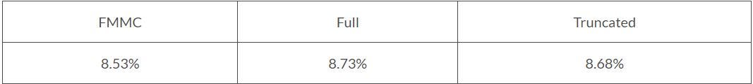
The table below depicts the mean (i.e. average) annual return for the factor model Monte Carlo (FMMC), full history of AHF (January 2010-March 2020) and the truncated/”observed” history (January 2017-March 2020):

下表描述了因子模型蒙特卡洛(FMMC)，AHF的完整历史记录(2010年1月至2020年3月)和截断/“观察到的”历史记录(2017年1月至2020年3月)的平均(即平均)年收益：

Immediately we can see the improvement that the FMMC model has over the Truncated period. The FMMC model is able to fully capture the return dynamic of AHF while the Truncated return substantially underestimates full history mean.

马上我们可以看到FMMC模型在截断期间的改进。 FMMC模型能够完全捕获AHF的返回动态，而截断的返回则大大低估了整个历史均值。

2. Volatility

2.波动性

Accurate estimation of the mean alone cannot support the claim that our model is robust. Of equal importance is the volatility. The below table shows the annualized volatility (i.e. standard deviation) for each of the periods under consideration:

仅凭均值的准确估计就不能支持我们的模型稳健的说法。 波动同样重要。 下表显示了所考虑的每个时期的年度波动率(即标准差)：

Both the FMMC and Truncated estimates slightly undershoot the realized volatility of AHF over the full period. However, both estimated are very close.

FMMC和“截断”估计都略微低于AHF在整个时期内已实现的波动性。 但是，两者估计都非常接近。

3. Sharpe Ratio

3.夏普比率

With the mean and volatility estimates in hand, we can now calculate the Sharpe Ratio. The Sharpe Ratio is calculated as follows:

有了平均值和波动率估算值，我们现在可以计算夏普比率。 夏普比率计算如下：

For most of the test period (January 2010-March 2020) the risk-free rate as proxied by the yield on the 3-month T-Bill was very close to 0%. For simplicity we will adopt 0% as the risk-free rate for our calculations. The below table shows the results:

在大多数测试期间(2010年1月至2020年3月)，由3个月国库券收益率所代表的无风险利率非常接近0％。 为简单起见，我们将采用0％作为无风险利率进行计算。 下表显示了结果：

The FMMC estimate shows dramatic improvement over the Truncated for estimating the Sharpe Ratio of AHF. This is not necessarily surprising as above we showed the mean return for the Truncated period to be poor while the estimate for the FMMC was quite close. Naturally this will feed into the results for Sharpe, but, again, the results show the utility of the FMMC approach.

FMMC估计值比截断值(用于估计AHF的Sharpe比率)显着提高。 这不一定是令人惊讶的，因为上面我们显示了截断期的平均收益很低，而FMMC的估算却非常接近。 自然，这将被纳入Sharpe的结果中，但是结果再次显示了FMMC方法的实用性。

4. Sortino Ratio

4. Sortino比率

Finally, we turn to the Sortino Ratio. Sortino is similar to Sharpe, but instead of total volatility, it is focused on what is termed “downside volatility”; or the standard deviation of returns below a stated threshold. Typically, the threshold is set to 0%; the idea being that volatile, positive returns are not considered “bad” because you are still making money, but volatile negative returns suggest an outsized chance of large losses. A higher ratio is considered better. The Sortino Ratio is calculated as follows:

最后，我们转到Sortino比率。 Sortino与Sharpe类似，但不是总波动率，而是着眼于所谓的“下行波动率”。 或低于规定门槛的收益标准偏差。 通常，阈值设置为0％； 之所以这样的想法是，因为您仍在赚钱，所以波动的正收益不被认为是“坏”的，但是波动的负收益表明出现巨额亏损的可能性很大。 比率越高越好。 Sortino比率计算如下：

The table depicts the results:

下表描述了结果：

The FMMC estimate is very close to the full period and accurately expresses the volatility of the downside returns. We see marked improvement over the Truncated estimate which is lower due to a combination of a lower average return and more downside volatility.

FMMC的估计非常接近整个周期，并准确表示了下行收益的波动性。 我们看到，由于平均收益较低和下行波动较大，两者的总和比截断后的估计要低得多。

结论性意见 (Concluding Comments)

Manager evaluation is one of the oldest and most common problems in investment finance. When the track record of the manager is short it can be difficult to assess the efficacy of the strategy which has ramifications for both fund managers and fund allocators.

经理评估是投资金融中最古老，最常见的问题之一。 如果经理的业绩记录很短，则可能难以评估该策略的有效性，这对基金经理和基金分配者都有影响。

In this post, we introduced Factor Model Monte Carlo (FMMC) as a possible solution to the short history problem and used the real world example of Aric’s Hedge Fund (AHF) to demonstrate its efficacy. By using a factor model and the common, short history of fund and factor returns, we estimated the exposure of AHF to different sources of economic and market risk. We were then able to simulate the returns of the AHF to construct a longer history of returns with the goal of gaining improved insight into the fund’s long term performance.

在本文中，我们介绍了因素模型蒙特卡洛(FMMC)作为短期历史问题的可能解决方案，并使用了Aric对冲基金(AHF)的真实示例来证明其有效性。 通过使用因子模型以及常见的短期资金和因子收益历史，我们估计了AHF暴露于不同的经济和市场风险来源的风险。 然后，我们能够模拟AHF的收益，以构建更长的收益历史，目的是获得对基金长期业绩的更深入了解。

The results from the FMMC method showed dramatic improvement over using the short history of returns in isolation. Using the full history of returns for AHF as a comparison, we see that the FMMC method accurately models the return, volatility, Sharpe and Sortino Ratios of the fund. By comparison, the truncated history of returns severely underestimated the performance of AHF which would have the consequence of misleading investors.

FMMC方法的结果表明，与单独使用较短的收益历史相比，有了显着的改进。 使用AHF的全部收益历史作为比较，我们可以看到FMMC方法可以准确地模拟基金的收益，波动率，夏普和Sortino比率。 相比之下，截短的收益历史严重低估了AHF的业绩，这可能会误导投资者。

Factor Model Monte Carlo has proven to be an effective technique for modeling risk and return for complex strategies and serves as a powerful addition to the fund analyst’s tool kit.

因子模型蒙特卡洛(Monte Carlo)已被证明是对复杂策略的风险和回报建模的有效技术，并且是基金分析师工具包的有力补充。

Until next time, thanks for reading!

直到下一次，感谢您的阅读！

Aric Lux.

阿里克斯·勒克斯(Aric Lux)。

Originally published at http://lightfinance.blog on August 28, 2020.

最初于 2020年8月28日 发布在 http://lightfinance.blog 上。