Clustering with R

用R聚类

本文是关于使用流行的“ Iris”数据集进行R中的动手集群分析(无监督机器学习)的。 (This article is about hands-on Cluster Analysis (an Unsupervised Machine Learning) in R with the popular ‘Iris’ data set.)

Let’s brush up some concepts from Wikipedia

让我们回顾一下维基百科的一些概念

Machine learning is the study of computer algorithms that improve automatically through experience. It is seen as a subset of Artificial Intelligence. Machine learning algorithms build a mathematical model based on sample data, in order to make predictions or decisions without being explicitly programmed to do so.

机器学习是对计算机算法的研究，这些算法会根据经验自动提高。 它被视为人工智能的子集。 机器学习算法会基于样本数据构建数学模型，以便做出预测或决策而无需明确地编程。

Supervised Learning is the machine learning task of learning a function that maps an input to an output based on example input-output pairs. It infers a function from labeled training data consisting of a set of training examples.

监督学习是机器学习任务，它学习基于示例输入输出对将输入映射到输出的功能。 它从标记的训练数据(由一组训练示例组成)中推断出功能。

Unsupervised Learning is a type of machine learning that looks for previously undetected patterns in a data set with no pre-existing labels and with a minimum of human supervision.

无监督学习是一种机器学习，它在没有预先存在的标签且最少需要人工监督的情况下，在数据集中查找先前未检测到的模式。

Cluster Analysis or Clustering is the task of grouping a set of objects in such a way that objects in the same group (called a cluster) are more similar (in some sense) to each other than to those in other groups (clusters).

聚类分析或聚类是，在所述相同的组(称为簇 )对象这样的方式，而不是那些在其他组(簇状物)的分组的一组物体更相似(在某些意义上)彼此的任务。

About Iris Data set

关于虹膜数据集

Iris flower data set was introduced by the British statistician and biologist Ronald Fisher in his 1936 paper The use of multiple measurements in taxonomic problems. This is perhaps the best known database to be found in the pattern recognition literature. Iris data set gives the measurements in centimetres of the variables sepal length and width and petal length and width, respectively, for 50 flowers from each of 3 species of iris. The species are Iris setosa, versicolor, and virginica.

鸢尾花数据集由英国统计学家和生物学家罗纳德·费舍尔 ( Ronald Fisher)在其1936年发表的论文中介绍。 这也许是模式识别文献中最著名的数据库。 鸢尾花数据集以厘米为单位，分别测量了3种鸢尾花中每种花的50朵花的萼片长度和宽度以及花瓣长度和宽度 。 该品种是山鸢尾， 花斑癣和弗吉尼亚 。

So, let’s start now ! You may like to download the Iris Data set & the R-script from my github repository.

所以，让我们开始吧！ 您可能想从我的github存储库 下载 Iris数据集和R脚本。

Hope you have R & RStudio installed for a hands-on experience with me :)

希望您已安装R ＆ RStudio，以便与我亲身体验:)

Objective

目的

The Objective is to segment the iris data(without labels) into clusters — 1, 2 & 3 by k-means clustering & compare these clusters with the actual species clusters — setosa, versicolor, and virginica.

目的是通过k均值聚类将虹膜数据(不带标签)分割为1、2和3类，并将这些类群与实际物种类群(setosa，versicolor和virginica)进行比较。

Install and Load R Packages

安装和加载R软件包

‘tidyverse’, ‘cluster’ and ‘reshape2’ — these three R packages are required here. Install if not done earlier. We need to load the packages with the library function.

'tidyverse'，'cluster'和'reshape2'-这三个R软件包在这里是必需的。 如果没有更早安装，请安装。 我们需要使用库函数加载软件包。

install.packages(“tidyverse”)       # for data work & visualizationinstall.packages(“cluster”)         # for cluster modeling install.packages("reshape2")        # for melting data# note : not required if already installedlibrary(tidyverse)library(cluster)library(reshape2)

Import the Iris Data set

导入虹膜数据集

We can import from disc after setting the working directory where the csv file is.

我们可以在设置csv文件所在的工作目录后从光盘导入。

setwd(“E:/my_folder/work_folder”)mydata <- read.csv(“iris.csv”)

Or, get it from the in-build R datasets

或者，从内置R数据集中获取它

mydata <- iris

Explore the Data set

探索数据集

With below functions we can check the data set before exploring

通过以下功能，我们可以在探索之前检查数据集

glimpse(mydata)head(mydata)View(mydata)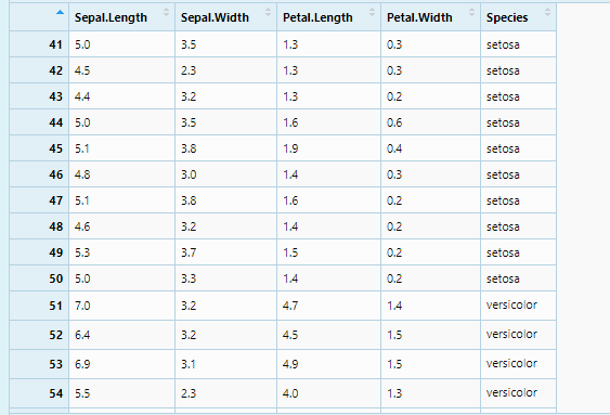

Let’s visualize the data now with ggplot2

现在使用ggplot2可视化数据

Sepal-Length vs. Sepal-Width

隔片长度与隔片宽度

ggplot(mydata)+ geom_point(aes(x = Sepal.Length, y = Sepal.Width), stroke = 2)+ facet_wrap(~ Species)+  labs(x = ‘Sepal Length’, y = ‘Sepal Width’)+ theme_bw()

Petal-Length vs. Petal-Width

花瓣长度与花瓣宽度

ggplot(mydata)+ geom_point(aes(x = Petal.Length, y = Petal.Width), stroke = 2)+ facet_wrap(~ Species)+  labs(x = ‘Petal Length’, y = ‘Petal Width’)+ theme_bw()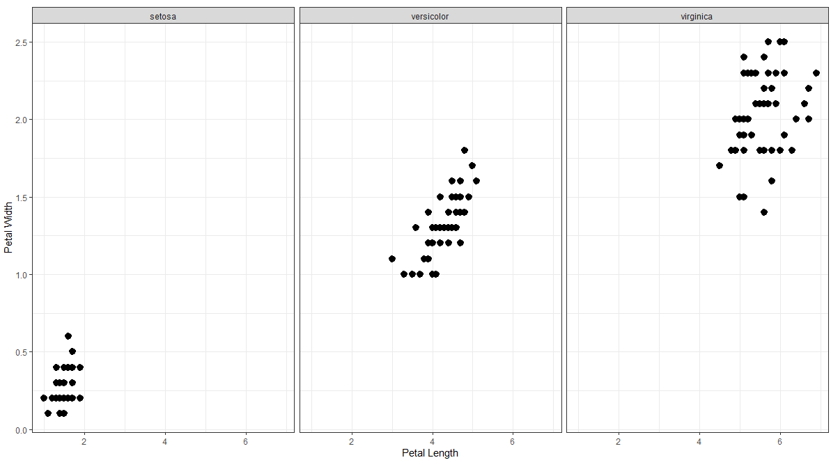

Sepal-Length vs. Petal-Length

Sepal-Length与Petal-Length

ggplot(mydata)+ geom_point(aes(x = Sepal.Length, y = Petal.Length), stroke = 2)+ facet_wrap(~ Species)+  labs(x = ‘Sepal Length’, y = ‘Petal Length’)+ theme_bw()

Sepal-Width vs. Pedal-Width

分隔宽度与踏板宽度

ggplot(mydata)+ geom_point(aes(x = Sepal.Width, y = Petal.Width), stroke = 2)+ facet_wrap(~ Species)+  labs(x = ‘Sepal Width’, y = ‘Pedal Width’)+ theme_bw()

Box plots

箱形图

ggplot(mydata)+ geom_boxplot(aes(x = Species, y = Sepal.Length, fill = Species))+ theme_bw()ggplot(mydata)+ geom_boxplot(aes(x = Species, y = Sepal.Width, fill = Species))+ theme_bw()ggplot(mydata)+ geom_boxplot(aes(x = Species, y = Petal.Length, fill = Species))+ theme_bw()ggplot(mydata)+ geom_boxplot(aes(x = Species, y = Petal.Width, fill = Species))+ theme_bw()

k均值聚类 (k-means Clustering)

k-means clustering is a method of vector quantization, that aims to partition n observations into k clusters in which each observation belongs to the cluster with the nearest mean (cluster centers or cluster centroid), serving as a prototype of the cluster.

k均值聚类是矢量量化的一种方法，旨在将n个观察值划分为k个聚类，其中每个观察值均属于具有最近均值(聚类中心或聚类质心 )的聚类，用作聚类的原型。

Find the optimal number of clusters by Elbow Method

用弯头法找到最优的簇数

set.seed(123) # for reproductionwcss <- vector()for (i in 1:10) wcss[i] <- sum(kmeans(mydata[, -5], i)$withinss)plot(1:10, wcss, type = ‘b’, main = paste(‘The Elbow Method’), xlab = ‘Number of Clusters’, ylab = ‘WCSS’)

the elbow point : k(centers) = 3

肘点： k(中心)= 3

Apply kmeans function to the feature columns

将 kmeans函数 应用于要素列

set.seed(123)km <- kmeans( x = mydata[, -5] , centers = 3)yclus <- km$clustertable(yclus)

output :

输出：

> table(yclus)yclus1  2  3 50 62 38

the kmeans has grouped the data into three clusters- 1, 2 & 3 having 50, 62 & 38 observations respectively.

kmeans已将数据分组为三个聚类，分别是具有50、62和38个观测值的1、2和3。

Visualize the kmeans clusters

可视化kmeans集群

clusplot(mydata[, -5], yclus, lines = 0, shade = TRUE, color = TRUE, labels = 0, plotchar = FALSE, span = TRUE, main = paste(‘Clusters of Iris Flowers’))

Compare the clusters

比较集群

mydata$cluster.kmean <- ycluscm <- table(mydata$Species, mydata$cluster.kmean)cm

output :

输出：

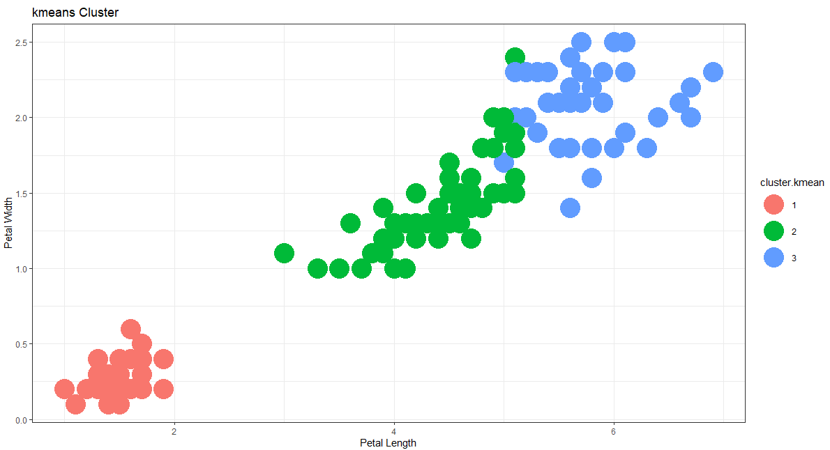
> cm1  2  3setosa       50 0  0versicolor   0  48 2virginica    0  14 36

[(50 + 48 + 36)/150] = 89% of the k-means cluster output matched with the actual Species clusters. versicolor(Cluster 2) & virginica(Cluster 3) have some overlapping features which is also apparent from the cluster visualizations.

[(50 + 48 + 36)/ 150] = 89个k均值群集输出与实际Species群集匹配。 versicolor(群集2)和virginica(群集3)具有一些重叠的功能，这在群集可视化中也很明显。

Tiles plot : Species vs. kmeans clusters

瓷砖图：物种vs. kmeans集群

mtable <- melt(cm)ggplot(mtable)+geom_tile(aes(x = Var1, y = Var2, fill = value))+ labs(x = ‘Species’, y = ‘kmeans Cluster’)+ theme_bw()

Scatter plots (to view Species & kmeans custers)

散点图(以查看物种和kmeans突击者)

Sepal-Length vs. Sepal-Width

隔片长度与隔片宽度

mydata$cluster.kmean <- as.factor(mydata$cluster.kmean)# Sepal-Length vs. Sepal-Width (Species)ggplot(mydata)+  geom_point(aes(x = Sepal.Length, y = Sepal.Width,                  color = Species) , size = 10)+   labs(x = 'Sepal Length', y = 'Sepal Width')+  ggtitle("Species")+  theme_bw()# Sepal-Length vs. Sepal-Width (kmeans cluster)ggplot(mydata)+  geom_point(aes(x = Sepal.Length, y = Sepal.Width,                  color = cluster.kmean) , size = 10)+   labs(x = 'Sepal Length', y = 'Sepal Width')+  ggtitle("kmeans Cluster")+  theme_bw()

Petal-Length vs. Petal-Width

花瓣长度与花瓣宽度

# Petal-Length vs. Petal-Width (Species)ggplot(mydata)+  geom_point(aes(x = Petal.Length, y = Petal.Width,                  color = Species) , size = 10)+   labs(x = 'Petal Length', y = 'Petal Width')+  ggtitle("Species")+  theme_bw()# Petal-Length vs. Petal-Width (kmeans cluster)ggplot(mydata)+  geom_point(aes(x = Petal.Length, y = Petal.Width,                  color = cluster.kmean) , size = 10)+   labs(x = 'Petal Length', y = 'Petal Width')+  ggtitle("kmeans Cluster")+  theme_bw()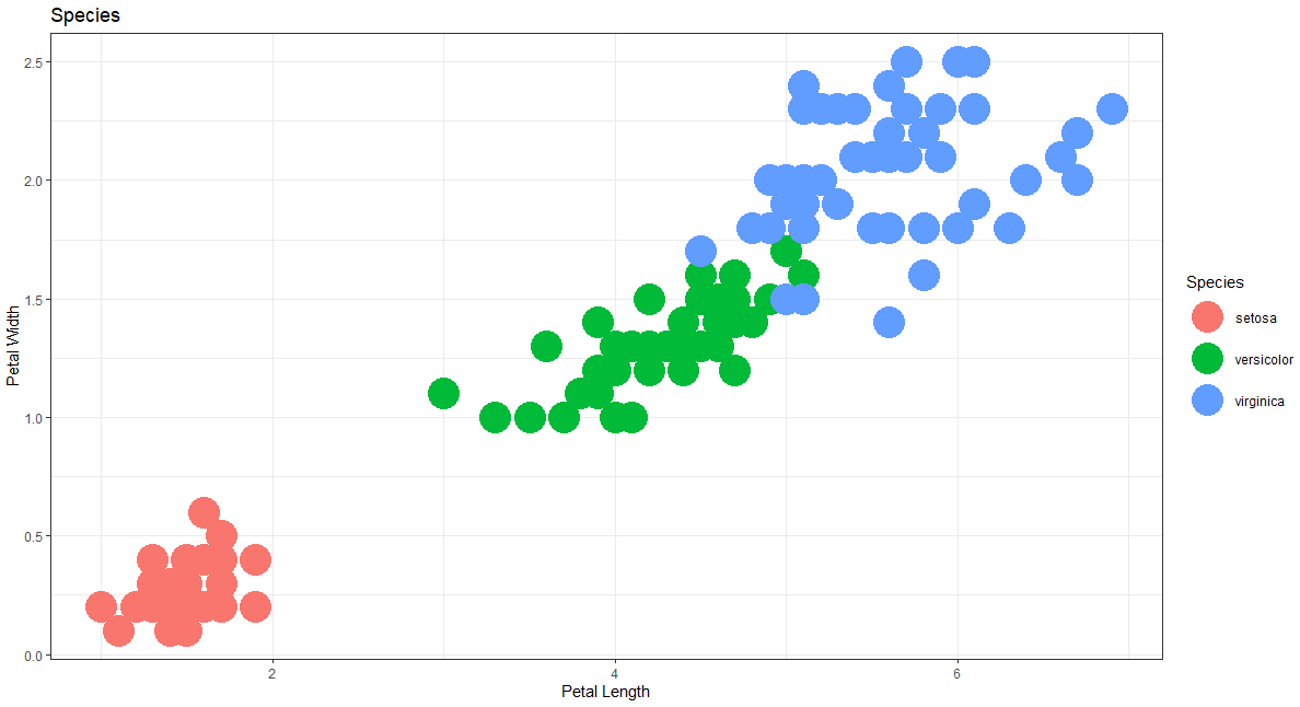

Hope you enjoyed the cluster analysis in R with interesting visualizations. Feel free to comment for any remark, suggestion or topic that you like me to write on.

希望您通过有趣的可视化方法喜欢R中的聚类分析。 对于您喜欢我写的任何评论，建议或主题，请随时发表评论。

This happened to be my first Medium article. A many more will come as I progress through the ladder of data science and machine learning fields. Keep calm and stay with me !

这恰好是我的第一篇中型文章。 随着我在数据科学和机器学习领域的发展，将会有更多的发展。 保持冷静，和我在一起！

Let’s ace data !!

让我们获得数据！