组合保险策略及相应模拟测算工具----Discrete Hedging: Guaranteed CPPI Structures

最近将 open code 稍作修改做了一个CPPI模拟测算工具，http://www.mathworks.com/matlabcentral/fileexchange/loadCategory.do?objectId=3&objectType=Category！

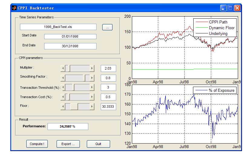
操作界面：

风险放大倍数、平滑因子、转换成本可以调整

相关CPPI 结构知识（摘自维基百科）

Discrete Hedging: Guaranteed CPPI Structures

1 Introduction...................................................................................................................................... 2

1.1 Discrete Hedging Risks......................................................................................................................... 2

1.2 CPPI Structures........................................................................................................................................ 3

1.3 Jump Diffusion............................................................................................................................................ 3

1.4 The Real Rate of Return...................................................................................................................... 4

2 Contract Specifications.......................................................................................................... 4

2.1 Trigger Level............................................................................................................................................ 4

2.2 Asset Allocation Table........................................................................................................................ 4

2.3 Effective Underlying Unit Value.................................................................................................... 4

2.4 Payment at Maturity............................................................................................................................ 5

2.5 Liquidity Features of the Underlying Fund............................................................................... 5

2.6 Features Not Dealt with by the Modelling............................................................................... 7

2.6.1 Uncertain Realised NAV Values........................................................................................................ 7

2.6.2 Different Purchase and Redemption Notice Dates........................................................................ 7

2.6.3 Different Borrowing and Lending Rates......................................................................................... 7

2.6.4 Investment Guidelines......................................................................................................................... 7

2.6.5 Termination Events.............................................................................................................................. 7

3 Market Data........................................................................................................................................ 7

4 Monte Carlo Pricing.................................................................................................................... 7

4.1 The Jump-Diffusion Process for A_t..................................................................................................... 8

4.2 The Outputs................................................................................................................................................ 8

5 References........................................................................................................................................... 9

1 Introduction

Mutual funds, hedge funds and funds of funds have a number of features that are markedly different to regular equity underlyings:

1. They can only be traded at discrete times. For example, mutual funds are often only tradable once a day. Some hedge funds or funds of funds can only be traded on a weekly, or monthly basis.[1]

2. Frequently notice has to be given before one intends to trade. For example, 5 days notice has to be given before purchasing, while 30 days notice has to be given before selling the fund.

3. One might agree on a value to trade, rather than a number of fund units to trade.

4. When purchasing of the fund cash might have to be delivered several days before trading, while on redeeming a part of the investment in the fund, it might take several days to weeks for delivery of the proceeds.

5. One might be limited in the volume that can be traded on a given day.

For pricing and risk management the first feature is frequently the most significant and is discussed below in section 1.1. One of the more frequently used structures to reduce the risks carried by the issuer is the CPPI (constant-proportions-portfolio-insurance) structure (see section 1.2). Only being able to trade at specific times raises the impact of sharp market moves – in the case of continuous hedging one can often hedge large up and down moves while they are occurring, whilst in the case of discrete hedging the full impact of large moves is experienced. Consequently we have extended the stock evolution to include additional random jumps – this is discussed more fully in section 1.3. The discrete nature also means that the relevant growth rate is not the risk-free rate, but rather the real rate of return – this is discussed more fully in section 1.4.

1.1 Discrete Hedging Risks

In a continuously tradable B&S world the fair price and the cost of the delta hedge are equal. In the case of discrete hedging this is no longer the case. It is simple to show that the discrete delta hedge might cost more than the equivalent continuous hedge. Consider the hedging of a call option over a month where the price of the underlying rises steadily:

1. In the case of continuous hedging one steadily buys more delta.

2. In the case of discrete monthly hedging one can only increase delta at the end of the month, which means that one must buy the additional delta at the highest price over the month, rather than on the way up.

In the case of the price dropping continuously over a month the discrete delta also costs more as one is forced to sell at the lowest point.

So when does the discrete case cost less than the continuous hedge? Consider the above case, with the modification that the underlying goes up and then returns to its original level by the end of the month. If one compares monthly hedging with bimonthly hedging we know that bimonthly hedging will cost something on the way up, and then something on the way down. In contrast monthly hedging will be approximately free.

Considering all the possible paths one ends up with a distribution for the costs of the delta hedge. The average of this distribution is the continuous B&S fair price. The more frequent the re-hedging times, the narrower the distribution of delta hedging costs. The main unhedgeable exposure is one’s gamma exposure; namely that one is limited in one’s ability to adjust the delta hedge.

A different view of the same problem is to consider a B&S world in which one considers a discrete path. The volatility of the discrete path will be distributed around the B&S volatility.[2] Indeed the distribution of option prices can be determined from this distribution of the discrete volatilities (see M. Kamal research paper). One useful result is that the width of the distribution scales as Ödt, the discrete time-step (in case of a standard B&S assumption).

It is important to realise that this risk cannot be hedged. One can be lucky and make a profit, or unlucky and make a loss with respect to the B&S ‘fair’ price. Of course by taking sensible provisions with respect to the B&S ‘fair’ price the risk of loss for the bank can be significantly reduced.

1.2 CPPI Structures

CPPI structures are contracts in which the client carries much of the above discrete hedging risk. In the simplest case, the complete notional is initially invested in the fund. If the spot rises the holding is increased (i.e. levered) in a prescribed manner, while if the spot drops the leverage is reduced – all according to an allocation table.[3] As the leveraging is prescribed the discrete hedging risk is completely borne by the client.

One problem with simple CPPI certificate-like structures is that the client might loose money. This could be largely overcome by modifying the initial allocation and the leverage schedule, but this usually leads to relatively low participation rates (similar to standard capital protected notes, with call options). However, a more frequent approach to overcome this risk is to have a trigger level, which if breached leads to the remaining holding being converted to cash for the rest of the contract’s life. The trigger level is related to the discount factor in such a way that in most cases the amount of cash held will guarantee the return of the notional at maturity. However, there remains a liquidity gap risk, said differently; the trigger level might be breached so rapidly (with respect to the available liquidity) that the investment can not be sold in time to guarantee the minimum amount of cash. Consequently two extra contract features are introduced:

· The prescribed allocation schedule leads to a rapid reduction of the investment (rapid increase in cash holding) as the trigger level is approached. This means that the fraction of the initial investment that is exposed to the liquidity gap risk is reduced.

· A gap provision shifts the trigger level above the discount factor by a few percent, thereby providing a larger buffer and thus further reducing the gap risk.

Even with these two features there is no firm guarantee of the return of the notional at maturity, so the issuer frequently offers a guarantee to the client, and thus carries this residual risk, himself. Much of the modelling described in this document is related to understanding this risk.

1.3 Jump Diffusion

One of the main attractions of fund-of-funds is their low historic volatility. This means that large moves tend to be rare-events, something Monte Carlo simulation is not suitable for. However, it is exactly the consequences of these events that we are trying to understand. One approach is to ramp up the volatility well above its historic levels, but this approach can significantly distort the overall simulation and should only be done with care. Another approach is to introduce extra random jumps not contained in a lognormal model. This extra component of the diffusion process is a random Poisson process, which is characterised by an expected jump frequency, an expected jump size that could be generalised to a random distribution about the expected jump size.

1.4 The Real Rate of Return

In the well-known Black and Scholes’ approach we eliminate the real rate of return, m, from the picture by requiring continuous dynamic delta hedging of the derivative product. Consequently, the portfolio consisting in the derivative and its delta hedge grows with the risk-free rate. If the liquidity is limited so that continuous hedging is no more possible, then the real rate of return becomes important again.

To see this, consider a position on an underlying that can be hedged once a month. One can choose the delta hedge to be the present delta, or the delta one expects to have when one can hedge again, i.e. in one month’s time. If the position has a non-zero gamma (and then, theta), then the two are different. The amount they are different is partially determined by the expected change in the underlying spot, E[dS]:

E[dS] = E[S_t+_dt] - S_t = S_t e^m^dt - S_t @ S_t mdt

In the case of continuous hedging, the next hedging opportunity is immediate (dt ® 0 ), thus allowing continuous dynamic delta-hedging, and so the removal of exposure to the real rate of return.

2 Contract Specifications

In this section we describe the features of a typical guaranteed CPPI contract. We concentrate on the features included in the modelling and at the end briefly summarise the main features not dealt with in the modelling. We also include a sub-section describing the liquidity features of the underlying fund.

2.1 Trigger Level

At any given time, t, before maturity, T, the trigger level, L_t, is given by:

L_t = Z_t + C_t Eq. 2.1

where Z_t is the prevailing discount factor from t to T, and C_t is the time-dependent gap provision given by:

X% is usually around 1%. This cushion level is increasing with time, because of the increase in the gamma risk when we get close to expiry.

2.2 Asset Allocation Table

The performance of the effective underlying Unit Value (before accounting for fees [see Eq. 2.2]), U_t’, relative to its initial value, U₀, is denoted by P_t = U_t’ / U₀. The distance of the performance from the trigger level is given by D_t = P_t – L_t.

At any given time the fraction of the value invested in the underlying fund is denoted as W_t, which is uniquely determined from the allocation table that is effectively a piecewise constant function that maps D_t onto W_t.

2.3 Effective Underlying Unit Value

The effective underlying unit value, U_t, is related to its previous value, U_t-1, and present Net Asset Value (NAV) of the underlying fund, A_t, and the previous NAV of the underlying fund, A_t-1, as follows:

Eq. 2.2

Where F_t is the risk monitoring fee for the following period (typically about 1% p.a. and charged on a monthly basis). This fee is proportional to U_t – it should be noted that F_t is unaffected by asianing.

Finally B_t is the cash holding and reflects either the non-invested cash or the borrowing for leverage. It is determined as:

It should be remembered that this cost of borrowing and lending includes the cost due to payment lags for redemption and early payment for purchase (see subsection 2.5).

U₀ = A₀ initialises Eq. 2.2.

2.4 Payment at Maturity

If no trigger event occurs then the payment at maturity is:

while if a trigger event has occurred the payment at maturity is given by:

where P_TE is the performance of the underlying unit value on the trigger event date, Z_TE is the prevailing discount factor on the trigger event date, and UnpaidFees_TE are the remaining risk monitoring fees on the trigger event date.

2.5 Liquidity Features of the Underlying Fund

Many funds have restrictive trading rules – the rule of thumb is that the restriction is there to benefit the fund. We list the four most important:

· Trading is restricted to weekly, or maybe monthly dates (however, estimated Net Asset Values are often given more frequently).

· Advance notice of purchase and sales must be given. Usually more notice is required for selling rather than buying.

· The volume traded on any one trading date might be limited – this can impact the initial delta hedge, or its sale at maturity. The problem at maturity can partially be overcome by averaging the final spot, which spreads the sale of the delta hedge out over several dates. The problem at start is less of a problem because (a) it is a purchase of the fund, and (b) the fund can be informed in advance of our intentions.

· The volume bought or sold might be quoted in value rather than units. The difference between the two is significant because of the notice period required.

In the picture below we illustrate the dates ‘associated’ with a given ‘Trading date’.

· An estimated NAV is reported by the fund. On this date the delta position is determined. Notice is given of one’s intention to purchase or redeem the fund.

· For purchases the money is handed over on the purchase payment date (no interest is accrued).

· The NAV is quoted on the trading date.

· Then come a series of redemption payment dates (only 2 are shown here). On each of these dates a fraction of the amount redeemed is received (without interest).

Purchase Payment Date

Time

Redemption Payment Date 1

Redemption Payment Date 2

Notice Date

Estimated NAV

Trading Date

Official NAV reported.

2.6 Features Not Dealt with by the Modelling

3 Market Data

Given the lack of tradable instruments on the underlying funds, we make many assumptions about the market data. Further, if there is any doubt, the assumptions nearly always tend to be conservative. Moreover, one can easily track the sensitivities with respect to non-hedgeable parameters and take that into account for both pricing and hedging.

1. Volatility is assumed to be flat. If it is available, a historical analysis of the fund’s NAV gives a range of volatilities. Typically, the volatility chosen for pricing is towards the top of this range, while the volatility for hedging is lower.

2. There are no dividends, but there are monitoring fees (F_t in Eq. 2.2).

3. The real rate of return is estimated from historical data of the fund.

4. The parameters for the jumps are estimated from historical data by looking at the moves (their size and frequency) which are too large to be considered compatible with the volatility otherwise exhibited.

4 Monte Carlo Pricing

The path-dependence of CPPI derivatives is strong, so Monte Carlo is the only tool that can price these options with all their bells and whistles; for example, in order to correctly account for the liquidity restrictions of the underlying fund. However, the weaknesses of Monte Carlo should be remembered: while it is good at average properties, analysis relying on tail properties must be treated with caution, and it must be remembered that modifications which boost the importance of tails will most probably distort other features as well.

The basic procedure is simple: Monte Carlo paths for the underlying fund, A_t, are generated until maturity. Equation 2.2 is then iteratively evolved to give the series for the underlying unit value, U_t. At maturity the position is liquidated and the proceeds are returned.

More specifically: the set of dates for the simulation of A_t is every trading day and its associated notice day. On every notice date the weight, W_t, is determined from the allocation table.[4] On every trading date, this weight and the actual NAV are used to determine the effective underlying unit value U_t from Eq. 2.2, remember the cost of funding purchases and the lags in receiving redemption.[5]

4.1 The Jump-Diffusion Process for A_t

The standard lognormal diffusion process is augmented with a jump process modelled by a Poisson process. A Poisson process is defined by a frequency (intensity) parameter, l, which determines the probability of an event in a short time as, ldt. The total process for the evolution of A_t becomes:

where a single jump size, J, is assumed – this size could also be made to be random, but given all the other assumptions, it seems excessive to include even more unknowns (we use conservative assumptions).

Note the use of the adjusted real rate of return, m’, which accounts for the drift effect of jumps:

4.2 The Outputs

The tool gives several outputs, coming from the Monte-Carlo simulations. The price gives the expected (discounted) value of the CPPI product. For a put, we give the price of the guarantee. For a call, we give the expected CPPI returns. Note that since we deal with the historical diffusion (and then, a drifting process), this value is not equal to the initial investment: it will be often slightly higher (thanks to the expected excess drift), even if the fees can lower it. From a theoretical point of view, this is compatible with the fact that, by dealing with the true probability, the important feature is the pair (expected returns vs. risk), and not only the price.

However, there is no really standard measure of the risk taken for derivative contracts. The VaR is not necessarily considering the tail events at their true value. This is why we give two different measures of risk to the user. The information is given in a histogram file (HISTOGRAM.txt), which can be retrieved on the Trade Spreadsheet.

The first one is the standard Value at Risk, based on the density distribution of the discounted flows, coming from the Monte-Carlo simulations. The second one is a weighted price distribution. Indeed, the risk aversion of the trader gives more value to potential losses than to potential gains. Instead of equally weighted probabilities, we can use a different pricing method: the more the loss, the more the weight.

Therefore, the VaR can actually be defined as the level such that: , and then:
,
whereas the other indicator is:

If we look at the upper tail (i.e. if the costs are higher than the average), C_i’ is higher than C_i. The second measure is therefore more conservative.

Since the distribution is given by a histogram, which synthesises the information on discrete points, the risk measure is sometimes slightly imprecise. You can choose the probability points that interest you (for the second measure only) under the “Std Deviation” cell. If you want the whole Monte-Carlo distribution (to manipulate the data by yourself), you shall type a negative number as a first point. The discounted prices for each trajectory are then filled in another output text file (namely, PRINT.txt).

5 References

· Kamal, M., ‘When You Cannot Hedge Continuously: The Corrections to Black-Scholes’, Goldman Sachs Equity Derivatives Research.

[1] Indeed even this limited liquidity can be reduced at the fund’s discretion, but for our purpose this is usually viewed as an early termination event.

[2] See ‘Volatility Capping’ (Steiner, M.)

[3] The client pays for the cost of leveraging or receives risk-free interest on non-invested cash.

[4] In principle the weight determined on the notice date should come from the expected value of the estimated NAV on the next trade date, and the expected trigger level on the next trade date.

[5] A_t-1 in Eq. 2.2 should be understood as the NAV on the previous trade date.

组合保险策略及相应模拟测算工具----Discrete Hedging: Guaranteed CPPI Structures相关推荐

组合保险策略模拟之基础知识
组合保险策略主要分为基于期权的投资组合保险(Option-Based Portfolio Insurance, OBPI)策略和固定比例投资组合保险 (Constant Proportion ...
保本基金的投资组合保险策略运用及建议
保本基金的投资组合保险策略运用及建议李源海摘要:保本基金的运作核心是投资组合保险策略,我国保本基金均采用简单参数的组合保险策略.在国内零息债券缺乏.股市波动大的情况下,如何设定最低保险额度.合理的 ...
基金公司业务突围策略探析——产品布局+工具化定位
基金公司业务突围策略探析--产品布局+工具化定位原创: 高道德.陈瑶海通量化团队 3天前重要提示:<证券期货投资者适当性管理办法>于2017年7月1日起正式实施,通过本微信订阅号发布 ...
python比较数据工具_Python模拟数据工具哪些比较好用
今天给大家推荐两款基本的Python模拟数据工具:mock和pytest monkeypatch. 为什么要模拟数据? 我们的应用中有一些部分需要依赖外部的库或对象.为了隔离开这部分,我们需要代替这些 ...
Python水滴筹模拟筹款工具
import timeprint(" 欢迎使用水滴筹模拟筹款工具 ") print("========================================== ...
java 驱动级模拟键盘,易语言开源驱动级模拟键盘工具（可绕过wegame屏蔽）
易语言开源驱动级模拟键盘工具目前一个可以绕过腾讯检测的模拟键盘工具,使用易语言开发,内含开源模块,支持调式修改,有需要模拟键盘的同学可以下载这个驱动模拟键盘来无视腾讯的wegame屏蔽! 相关阅读手 ...
一些前端模拟接口工具和相关文章
一些前端模拟接口工具最近在编写一些组件,需要模拟接口返回数据,所以收集一些常用的模拟接口工具,供日常学习使用,有新的也会更新记录 https://designer.mocky.io/ https:/ ...
移动端模拟开发者工具Eruda
移动端模拟开发者工具Eruda 前言:Eruda 是一个专为手机网页前端设计的调试面板,类似 DevTools 的迷你版,其主要功能包括:捕获 console 日志.检查元素状态.捕获XHR请求.显示 ...
Java之GUI编程学习笔记六 —— AWT相关（画笔paint、鼠标监听事件、模拟画图工具）
Java之GUI编程学习笔记六 -- AWT相关(画笔paint) 参考教程B站狂神https://www.bilibili.com/video/BV1DJ411B75F 了解paint Frame自 ...