Logistic regression is one of the most used machine learning techniques. Its main advantages are clarity of results and its ability to explain the relationship between dependent and independent features in a simple manner. It requires comparably less processing power, and is, in general, faster than Random Forest or Gradient Boosting.

逻辑回归是最常用的机器学习技术之一。 它的主要优点是结果清晰，并能够以简单的方式解释相关特征和独立特征之间的关系。 它所需的处理能力相对较小，并且通常比“随机森林”或“梯度增强”更快。

However, it has also some serious drawbacks and the main one is its limited ability to resolve non-linear problems. In this article, I will demonstrate how we can improve the prediction of non-linear relationships by incorporating a decision tree into a regression model.

但是，它也有一些严重的缺点，主要的缺点是解决非线性问题的能力有限。 在本文中，我将演示如何通过将决策树合并到回归模型中来改善非线性关系的预测。

The idea is quite similar to weight of evidence (WoE), a method widely used in finance for building scorecards. WoE takes a feature (continuous or categorical) and splits it into bands to maximise separation between goods and bads (positives and negatives). Decision tree carries out a very similar task, splitting the data into nodes to achieve maximum segregation between positives and negatives. The main difference is that WoE is built separately for each feature, while nodes of decision tree select multiple features at the same time.

这个想法与证据权重 (WoE)非常相似，证据权重 (WoE)是广泛用于构建记分卡的财务方法。 WoE具有一个特征(连续的或分类的)并将其划分为多个带，以最大程度地区分商品和不良商品(正面和负面)。 决策树执行非常类似的任务，将数据拆分为节点，以实现正负之间的最大隔离。 主要区别在于WoE是针对每个功能分别构建的，而决策树的节点同时选择多个功能。

Knowing that the decision tree is good at identifying non-linear relationships between dependent and independent features, we can transform the output of the decision tree (nodes) into a categorical variable and then deploy it in a logistic regression, by transforming each of the categories (nodes) into dummy variables.

知道决策树擅长识别依赖特征和独立特征之间的非线性关系，我们可以将决策树(节点)的输出转换为分类变量，然后通过转换每个类别将其部署到逻辑回归中(节点)转换为虚拟变量。

In my professional projects, using decision tree nodes in the model would out-perform both logistic regression and decision tree results in 1/3 of cases. However, I have struggled to find any publicly available data which could replicate it. This is probably because the available data contain only a handful of variables, pre-selected and cleansed. There is simply not much to squeeze! It is much easier to find additional dimensions of the relationship between dependent and independent features when we have hundreds or thousands of variables at our disposal.

在我的专业项目中，在模型中使用决策树节点将胜过逻辑回归和1/3情况下的决策树结果。 但是，我一直在努力寻找任何可以复制它的公开数据。 这可能是因为可用数据仅包含少数几个预先选择和清除的变量。 根本没有什么可挤压的！ 当我们拥有成百上千个变量时，查找从属特征和独立特征之间关系的其他维度要容易得多。

In the end, I decided to use the data from a banking campaign. Using these data I have managed to get a minor, but still an improvement of combined logistic regression and decision tree over both these methods used separately.

最后，我决定使用银行业务活动中的数据 。 通过使用这些数据，我设法取得了较小的成绩，但与单独使用的这两种方法相比，仍然改进了逻辑回归和决策树的组合。

After importing the data I did some cleansing. The code used in this paper is available on GitHub. I have saved the cleansed data into a separate file.

导入数据后，我进行了一些清理。 本文中使用的代码可在GitHub上获得。 我已将清理后的数据保存到一个单独的文件中 。

Because of the small frequency, I have decided to oversample the data using SMOTE technique.

由于频率较低，我决定使用SMOTE技术对数据进行过采样。

import pandas as pdfrom sklearn.model_selection import train_test_splitfrom imblearn.over_sampling import SMOTEdf=pd.read_csv('banking_cleansed.csv')X = df.iloc[:,1:]y = df.iloc[:,0]os = SMOTE(random_state=0)X_train, X_test, y_train, y_test = train_test_split(X, y, test_size=0.3, random_state=0)columns = X_train.columnsos_data_X,os_data_y=os.fit_sample(X_train, y_train)os_data_X = pd.DataFrame(data=os_data_X,columns=columns )os_data_y= pd.DataFrame(data=os_data_y,columns=['y'])

In the next steps I have built 3 models:

在接下来的步骤中，我建立了3个模型：

• decision tree决策树
• logistic regression逻辑回归
• logistic regression with decision tree nodes决策树节点的逻辑回归

Decision tree

决策树

It is important to keep the decision tree depth to a minimum if you want to combine with logistic regression. I’d prefer to keep the decision tree at maximum depth of 4. This already gives 16 categories. Too many categories may cause cardinality problems and overfit the model. In our example, the incremental increase in predictability between depth of 3 and 4 was minor, therefore I have opted for maximum depth = 3.

如果要与逻辑回归结合使用，则将决策树的深度保持在最低水平非常重要。 我希望决策树的最大深度保持为4。这已经给出了16个类别。 太多类别可能会导致基数问题并过拟合模型。 在我们的示例中，深度3和4之间的可预测性的增量增加很小，因此我选择最大深度= 3。

from sklearn.tree import DecisionTreeClassifierfrom sklearn import metricsfrom sklearn.metrics import roc_auc_scoredt = DecisionTreeClassifier(criterion='gini', min_samples_split=200,min_samples_leaf=100, max_depth=3)dt.fit(os_data_X, os_data_y)y_pred3 = dt.predict(X_test)print('Misclassified samples: %d' % (y_test != y_pred3).sum())print(metrics.classification_report(y_test, y_pred3))print (roc_auc_score(y_test, y_pred3))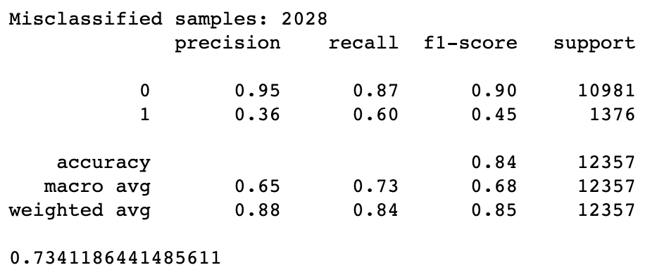

The next step is to convert the nodes into new variable. To do so, we need to code-up the decision tree rules. Luckily, there is a bit of programme which can do it for us. The function below produces a piece of code which is a replication of decision tree split rules.

下一步是将节点转换为新变量。 为此，我们需要对决策树规则进行编码。 幸运的是，有一些程序可以为我们做。 下面的函数生成一段代码，该代码是决策树拆分规则的复制。

from sklearn.tree import _treenn=0
def tree_to_code(tree, feature_names):tree_ = tree.tree_feature_name = [feature_names[i] if i != _tree.TREE_UNDEFINED else "undefined!"for i in tree_.feature]#print ("def tree({}):" .format(", " .join(feature_names)))def recurse(node, depth):indent = "    " * depthif tree_.feature[node] != _tree.TREE_UNDEFINED:table = 'X_train'name = table+"['"+feature_name[node]+"']"threshold = tree_.threshold[node]print ("{}if {} <= {}:".format(indent, name, threshold))recurse(tree_.children_left[node], depth + 1)print ("{}else:  # if {} > {}".format(indent, name, threshold))recurse(tree_.children_right[node], depth + 1)else:def increment():global nnnn=nn+1increment()print ("{}return 'Node_{}'".format(indent, nn))recurse(0, 1)

Now run the code:

现在运行代码：

tree_to_code(dt,columns)

and output will look like this:

输出将如下所示：

We can now copy and paste the output into our next function, which we can use to create our new categorical variable.

现在，我们可以将输出复制并粘贴到下一个函数中，使用该函数可以创建新的分类变量。

def tree(X_train):if X_train['nr_employed'] <= -0.9410539865493774:if X_train['pdays'] <= -5.0745530128479:if X_train['cons_price_idx'] <= -2.3744064569473267:return 'Node_1'else:  # if X_train['cons_price_idx'] > -2.3744064569473267return 'Node_2'else:  # if X_train['pdays'] > -5.0745530128479if X_train['loan_yes'] <= 0.5:return 'Node_3'else:  # if X_train['loan_yes'] > 0.5return 'Node_4'else:  # if X_train['nr_employed'] > -0.9410539865493774if X_train['cons_conf_idx'] <= -1.231077253818512:if X_train['cons_price_idx'] <= -0.8649553954601288:return 'Node_5'else:  # if X_train['cons_price_idx'] > -0.8649553954601288return 'Node_6'else:  # if X_train['cons_conf_idx'] > -1.231077253818512if X_train['default_unknown'] <= 0.5:return 'Node_7'else:  # if X_train['default_unknown'] > 0.5return 'Node_8'

Now we can quickly create a new variable (‘nodes’) and transfer it into dummies.

现在，我们可以快速创建一个新变量(“节点”)并将其转换为虚拟变量。

df['nodes']=df.apply(tree, axis=1)df_n= pd.get_dummies(df['nodes'],drop_first=True)df_2=pd.concat([df, df_n], axis=1)df_2=df_2.drop(['nodes'],axis=1)

After adding nodes variable, I re-run split to train and test groups and oversampled the train data using SMOTE .

添加节点变量后，我重新运行拆分以训练和测试组，并使用SMOTE对火车数据进行过采样。

X = df_2.iloc[:,1:]y = df_2.iloc[:,0]os = SMOTE(random_state=0)X_train, X_test, y_train, y_test = train_test_split(X, y, test_size=0.3, random_state=0)columns = X_train.columnsos_data_X,os_data_y=os.fit_sample(X_train, y_train)

Now we can run logistic regressions and compare the impact of node dummies on predictability.

现在，我们可以运行逻辑回归并比较节点虚拟变量对可预测性的影响。

Logistic regression excluding nodes dummies

逻辑回归排除节点假人

I have created a list of all features excluding the nodes dummies:

我创建了除节点虚拟变量之外的所有功能的列表：

nodes=df_n.columns.tolist()Init = os_data_X.drop(nodes,axis=1).columns.tolist()

and run the logistic regression using the Init list:

并使用“初始化”列表运行逻辑回归：

from sklearn.linear_model import LogisticRegressionlr0 = LogisticRegression(C=0.001, random_state=1)lr0.fit(os_data_X[Init], os_data_y)y_pred0 = lr0.predict(X_test[Init])print('Misclassified samples: %d' % (y_test != y_pred0).sum())print(metrics.classification_report(y_test, y_pred0))print (roc_auc_score(y_test, y_pred0))

Logistic regression with nodes dummies

节点假人的逻辑回归

In the next step I re-run the regression, but this time I have included nodes dummies.

在下一步中，我重新运行回归，但是这次我包括了节点虚拟对象。

from sklearn.linear_model import LogisticRegressionlr1 = LogisticRegression(C=0.001, random_state=1)lr1.fit(os_data_X, os_data_y)y_pred1 = lr1.predict(X_test)print('Misclassified samples: %d' % (y_test != y_pred1).sum())print(metrics.classification_report(y_test, y_pred1))print (roc_auc_score(y_test, y_pred1))

Results comparison

结果比较

The logistic regression with node dummies has the best performance. Although, the incremental improvement is not massive (especially if compared with decision tree), as I said before, it is hard to squeeze anything extra out data which contain only a handful of pre-selected variables and I can reassure you that in real life the differences can be bigger.

带有节点虚拟变量的逻辑回归具有最佳性能。 尽管增量改进并不大(特别是与决策树相比)，但正如我之前所说，很难挤出仅包含少量预选变量的额外数据，我可以向您保证差异可能更大。

We can scrutinise the models a little bit more by comparing the distribution of positives and negatives across the decile score using Model Lift, which I have presented in my previous article.

我们可以使用我在上一篇文章中介绍过的Model Lift比较正态分布和负分布在十分位得分上的分布情况，对模型进行更多的检查。

First step is to obtain probabilities:

第一步是获得概率：

y_pred0b=lr0.predict_proba(X_test[Init])y_pred1b=lr1.predict_proba(X_test)

Next we need to run the function below:

接下来，我们需要运行以下功能：

import numpy as np
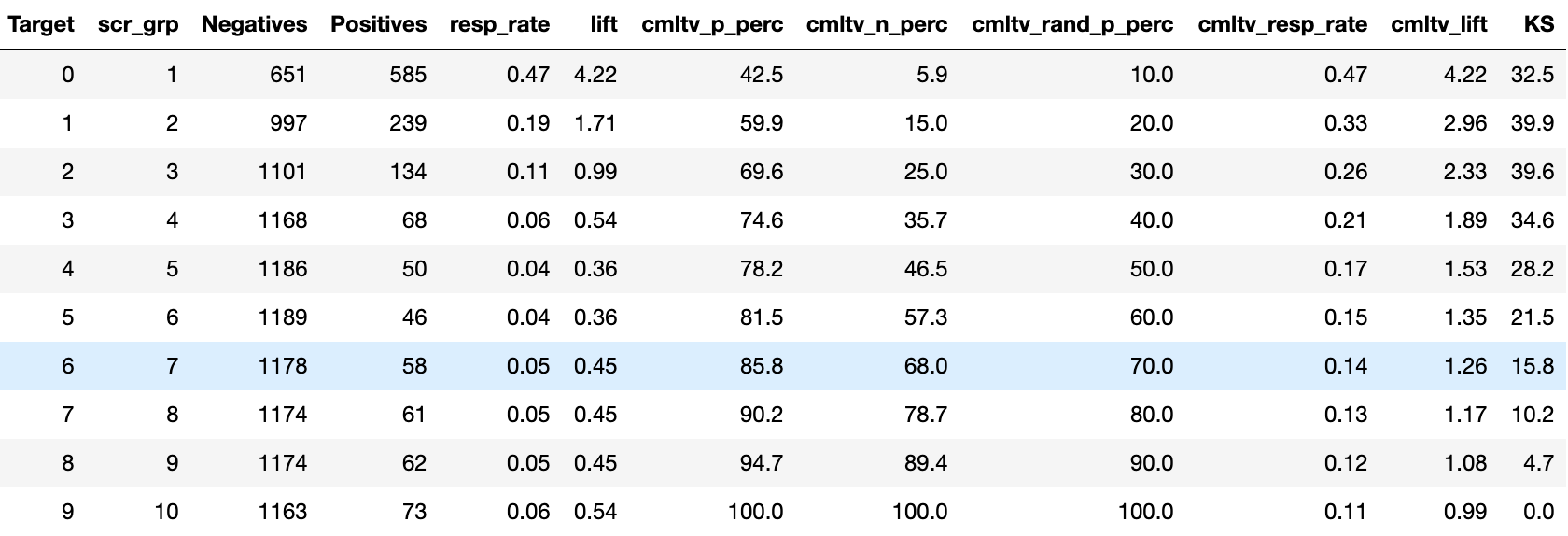
def lift (test, pred, cardinaility):res = pd.DataFrame(np.column_stack((test, pred)),columns=['Target','PR_0', 'PR_1'])res['scr_grp'] = pd.qcut(res['PR_0'], cardinaility, labels=False)+1crt = pd.crosstab(res.scr_grp, res.Target).reset_index()crt = crt.rename(columns= {'Target':'Np',0.0: 'Negatives', 1.0: 'Positives'})G = crt['Positives'].sum()B = crt['Negatives'].sum()avg_resp_rate = G/(G+B)crt['resp_rate'] = round(crt['Positives']/(crt['Positives']+crt['Negatives']),2)crt['lift'] = round((crt['resp_rate']/avg_resp_rate),2)crt['rand_resp'] = 1/cardinailitycrt['cmltv_p'] = round((crt['Positives']).cumsum(),2)crt['cmltv_p_perc'] = round(((crt['Positives']/G).cumsum())*100,1)crt['cmltv_n'] = round((crt['Negatives']).cumsum(),2)  crt['cmltv_n_perc'] = round(((crt['Negatives']/B).cumsum())*100,1)   crt['cmltv_rand_p_perc'] = (crt.rand_resp.cumsum())*100crt['cmltv_resp_rate'] = round(crt['cmltv_p']/(crt['cmltv_p']+crt['cmltv_n']),2)   crt['cmltv_lift'] = round(crt['cmltv_resp_rate']/avg_resp_rate,2)crt['KS']=round(crt['cmltv_p_perc']-crt['cmltv_rand_p_perc'],2)crt = crt.drop(['rand_resp','cmltv_p','cmltv_n',], axis=1)print('average response rate: ' , avg_resp_rate)return crt

Now we can check the differences between these two models. First, let’s evaluate the performance of the initial model without decision tree.

现在我们可以检查这两个模型之间的差异。 首先，让我们评估没有决策树的初始模型的性能。

ModelLift0 = lift(y_test,y_pred0b,10)ModelLift0

Model Lift before applying decision tree nodes…

在应用决策树节点之前进行模型提升…

…and next the model with decision tree nodes

…然后是带有决策树节点的模型

ModelLift1 = lift(y_test,y_pred1b,10)ModelLift1

Response in top 2 deciles of the model with decision tree nodes has improved, and so did the Kolmogorov-Smirnov test(KS). Once we translate the lift into financial value, it may turn out that this minimal incremental improvement may generate a substantial return in our marketing campaign.

具有决策树节点的模型的前两个十分之一的响应得到了改善，Kolmogorov-Smirnov检验(KS)也得到了改善。 一旦我们将提升转化为财务价值，就可以证明，这种最小的增量改进可能会在我们的营销活动中产生可观的回报。

Summarising, combining logistic regression and decision tree is not a well-known approach, but it may outperform the individual results of both decision tree and logistic regression. In the example presented in this article, the differences between decision tree and 2nd logistic regression are very negligible. However, in real life, when working on un-polished data, combining decision tree with logistic regression may produce far better results. That was rather a norm in projects I have run in the past. Node variable may not be a magic wand but definitely something worth knowing and trying out.

总结一下，将逻辑回归和决策树结合起来并不是一个众所周知的方法，但是它可能胜过决策树和逻辑回归的单独结果。 在本文提供的示例中，决策树和第二逻辑回归之间的差异非常小。 但是，在现实生活中，当处理未优化的数据时，将决策树与逻辑回归相结合可能会产生更好的结果。 那是我过去运行的项目中的一种规范。 Node变量可能不是魔杖，但绝对是值得了解和尝试的东西。