Note from Towards Data Science’s editors: While we allow independent authors to publish articles in accordance with our rules and guidelines, we do not endorse each author’s contribution. You should not rely on an author’s works without seeking professional advice. See our Reader Terms for details.

Towards Data Science编辑的注意事项： 尽管我们允许独立作者按照我们的 规则和指南 发表文章 ，但我们不认可每位作者的贡献。 您不应在未征求专业意见的情况下依赖作者的作品。 有关 详细信息， 请参见我们的 阅读器条款 。

With the recent volatility of the stock market due to the COVID-19 pandemic, I thought it was a good idea to try and utilize machine learning to predict the near-future trends of the stock market. I’m fairly new to machine learning, and this is my first Medium article so I thought this would be a good project to start off with and showcase.

鉴于最近由于COVID-19大流行而导致的股市波动，我认为尝试利用机器学习来预测股市的近期趋势是一个好主意。 我是机器学习的新手，这是我的第一篇中型文章，所以我认为这是一个很好的项目，首先要进行展示。

This article tackles different topics concerning data science, namely; data collection and cleaning, feature engineering, as well as the creation of machine learning models to make predictions.

本文讨论了与数据科学有关的不同主题，即： 数据收集和清理，功能工程以及创建机器学习模型以进行预测。

Author’s disclaimer: This project is not financial or investment advice. It is not a guarantee that it will provide the correct results most of the time. Therefore you should be very careful and not use this as a primary source of trading insight.

作者免责声明：该项目不是财务或投资建议。 不能保证大部分时间都会提供正确的结果。 因此，您应该非常小心，不要将其用作交易洞察力的主要来源。

You can find all the code on a jupyter notebook on my github:

您可以在我的github上的jupyter笔记本上找到所有代码：

1.进口和数据收集 (1. Imports and Data Collection)

To begin, we include all of the libraries used for this project. I used the yfinance API to gather all of the historical stock market data. It’s taken directly from the yahoo finance website, so it’s very reliable data.

首先，我们包括用于该项目的所有库。 我使用yfinance API收集了所有历史股票市场数据。 它直接来自雅虎财经网站，因此它是非常可靠的数据。

import yfinance as yf
import datetime
import pandas as pd
import numpy as np
from finta import TA
import matplotlib.pyplot as pltfrom sklearn import svm
from sklearn.ensemble import RandomForestClassifier
from sklearn.neighbors import KNeighborsClassifier
from sklearn.ensemble import AdaBoostClassifier
from sklearn.ensemble import GradientBoostingClassifier
from sklearn.ensemble import VotingClassifier
from sklearn.model_selection import train_test_split, GridSearchCV
from sklearn.metrics import confusion_matrix, classification_report
from sklearn import metrics

We then define some constants that used in data retrieval and data processing. The list with the indicator symbols is useful to help use produce more features for our model.

然后，我们定义一些用于数据检索和数据处理的常量。 带有指示器符号的列表对于帮助使用为我们的模型产生更多功能很有用。

"""
Defining some constants for data mining
"""NUM_DAYS = 10000     # The number of days of historical data to retrieve
INTERVAL = '1d'     # Sample rate of historical data
symbol = 'SPY'      # Symbol of the desired stock# List of symbols for technical indicators
INDICATORS = ['RSI', 'MACD', 'STOCH','ADL', 'ATR', 'MOM', 'MFI', 'ROC', 'OBV', 'CCI', 'EMV', 'VORTEX']

Here’s a link where you can find the actual names of some of these features.

在此链接中，您可以找到其中某些功能的实际名称。

Now we pull our historical data from yfinance. We don’t have many features to work with — not particularly useful unless we find a way to normalize them at least or derive more features from them.

现在，我们从yfinance中提取历史数据。 我们没有很多功能可以使用-除非我们找到一种方法至少可以将它们标准化或从中获得更多功能，否则它就没有什么用处。

"""
Next we pull the historical data using yfinance
Rename the column names because finta uses the lowercase names
"""start = (datetime.date.today() - datetime.timedelta( NUM_DAYS ) )
end = datetime.datetime.today()data = yf.download(symbol, start=start, end=end, interval=INTERVAL)
data.rename(columns={"Close": 'close', "High": 'high', "Low": 'low', 'Volume': 'volume', 'Open': 'open'}, inplace=True)
print(data.head())tmp = data.iloc[-60:]
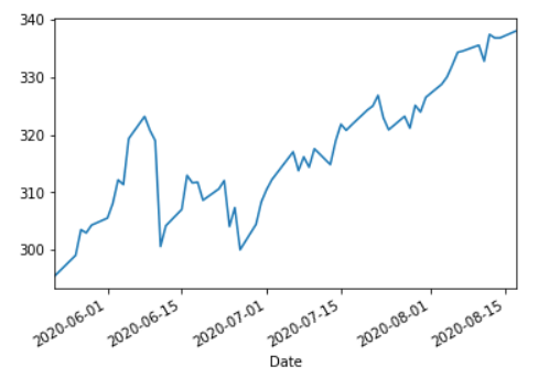
tmp['close'].plot()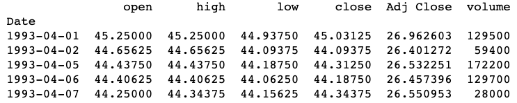

2.数据处理与特征工程 (2. Data Processing & Feature Engineering)

We see that our data above is rough and contains lots of spikes for a time series. It isn’t very smooth and can be difficult for the model to extract trends from. To reduce the appearance of this we want to exponentially smooth our data before we compute the technical indicators.

我们看到上面的数据是粗糙的，并且包含一个时间序列的许多峰值。 它不是很平滑，模型很难从中提取趋势。 为了减少这种情况的出现，我们希望在计算技术指标之前以指数方式平滑数据。

"""
Next we clean our data and perform feature engineering to create new technical indicator features that our
model can learn from
"""def _exponential_smooth(data, alpha):"""Function that exponentially smooths dataset so values are less 'rigid':param alpha: weight factor to weight recent values more"""return data.ewm(alpha=alpha).mean()data = _exponential_smooth(data, 0.65)tmp1 = data.iloc[-60:]
tmp1['close'].plot()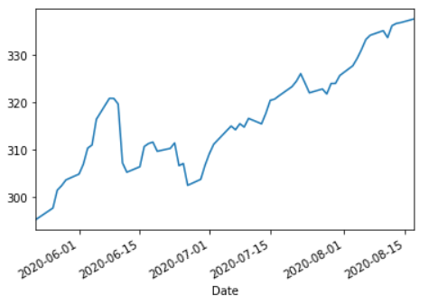

We can see that the data is much more smoothed. Having many peaks and troughs can make it hard to approximate, or be difficult to extract tends when computing the technical indicators. It can throw the model off.

我们可以看到数据更加平滑。 在计算技术指标时，具有许多波峰和波谷会使其难以估计或难以提取趋势。 它可能会使模型失效。

Now it’s time to compute our technical indicators. As stated above, I use the finta library in combination with python’s built in eval function to quickly compute all the indicators in the INDICATORS list. I also compute some ema’s at different average lengths in addition to a normalized volume value.

现在该计算我们的技术指标了。 如上所述，我结合使用finta库和python的内置eval函数来快速计算INDICATORS列表中的所有指标。 除了归一化的体积值，我还计算了不同平均长度下的一些ema。

I remove the columns like ‘Open’, ‘High’, ‘Low’, and ‘Adj Close’ because we can get a good enough approximation with our ema’s in addition to the indicators. Volume has been proven to have a correlation with price fluctuations, which is why I normalized it.

我删除了诸如“打开”，“高”，“低”和“调整关闭”之类的列，因为除指标外，我们还可以获得与ema足够好的近似值。 交易量已被证明与价格波动有关，这就是为什么我将其标准化。

def _get_indicator_data(data):"""Function that uses the finta API to calculate technical indicators used as the features:return:"""for indicator in INDICATORS:ind_data = eval('TA.' + indicator + '(data)')if not isinstance(ind_data, pd.DataFrame):ind_data = ind_data.to_frame()data = data.merge(ind_data, left_index=True, right_index=True)data.rename(columns={"14 period EMV.": '14 period EMV'}, inplace=True)# Also calculate moving averages for featuresdata['ema50'] = data['close'] / data['close'].ewm(50).mean()data['ema21'] = data['close'] / data['close'].ewm(21).mean()data['ema15'] = data['close'] / data['close'].ewm(14).mean()data['ema5'] = data['close'] / data['close'].ewm(5).mean()# Instead of using the actual volume value (which changes over time), we normalize it with a moving volume averagedata['normVol'] = data['volume'] / data['volume'].ewm(5).mean()# Remove columns that won't be used as featuresdel (data['open'])del (data['high'])del (data['low'])del (data['volume'])del (data['Adj Close'])return datadata = _get_indicator_data(data)
print(data.columns)

Index(['close', 'RSI', 'MACD', 'SIGNAL', '14 period STOCH %K','MFV', '14 period ATR', 'MOM', '14 period MFI', 'ROC', 'OBV_x', 'OBV_y', '20 period CCI', '14 period EMV', 'VIm', 'VIp', 'ema50', 'ema21', 'ema14', 'ema5', 'normVol'], dtype='object')

Right before we gather our predictions, I decided to keep a small bit of data to predict future values with. This line captures 5 rows corresponding to the 5 days of the week on July 27th.

在我们收集预测之前，我决定保留少量数据来预测未来价值。 该行捕获与7月27日一周中的5天相对应的5行。

live_pred_data = data.iloc[-16:-11]

Now comes one of the most important part of this project — computing the truth values. Without these, we wouldn’t even be able to train a machine learning model to make predictions.

现在是该项目最重要的部分之一-计算真值。 没有这些，我们甚至无法训练机器学习模型来进行预测。

How do we obtain truth value? Well it’s quite intuitive. If we want to know when a stock will increase or decrease (to make a million dollars hopefully!) we would just need to look into the future and observe the price to determine if we should buy or sell right now. Well, with all this historical data, that’s exactly what we can do.

我们如何获得真理价值？ 好吧，这很直观。 如果我们想知道什么时候股票会增加或减少(希望能赚到一百万美元！)，我们只需要展望未来并观察价格，以确定我们现在是否应该买卖。 好吧，有了所有这些历史数据，这正是我们所能做的。

Going back to the table where we initially pulled our data, if we want to know the buy (1) or sell (0) decision on the day of 1993–03–29 (where the closing price was 11.4375), we just need to look X days ahead to see if the price is higher or lower than that on 1993–03–29. So if we look 1 day ahead, we see that the price increased to 11.5. So the truth value on 1993–03–29 would be a buy (1).

回到我们最初提取数据的表，如果我们想知道1993-03-29日(收盘价为11.4375)当天的买入(1)或卖出(0)决定，我们只需要提前X天查看价格是否高于或低于1993-03-29的价格。 因此，如果我们提前1天查看价格，价格会升至11.5。 因此，1993-03-29年的真值将为购买(1)。

Since this is also the last step of data processing, we remove all of the NaN value that our indicators and prediction generated, as well as removing the ‘close’ column.

由于这也是数据处理的最后一步，因此我们删除了指标和预测生成的所有NaN值，并删除了“关闭”列。

def _produce_prediction(data, window):"""Function that produces the 'truth' valuesAt a given row, it looks 'window' rows ahead to see if the price increased (1) or decreased (0):param window: number of days, or rows to look ahead to see what the price did"""prediction = (data.shift(-window)['close'] >= data['close'])prediction = prediction.iloc[:-window]data['pred'] = prediction.astype(int)return datadata = _produce_prediction(data, window=15)
del (data['close'])
data = data.dropna() # Some indicators produce NaN values for the first few rows, we just remove them here
data.tail()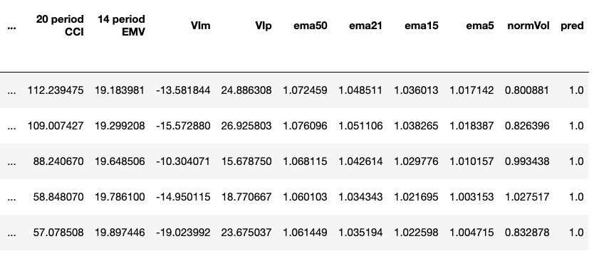

Because we used Pandas’ shift() function, we lose about 15 rows from the end of the dataset (which is why I captured the week of July 27th before this step).

因为我们使用了Pandas的shift()函数，所以从数据集的末尾损失了大约15行(这就是为什么我在此步骤之前于7月27日那周捕获了数据)。

3.模型创建 (3. Model Creation)

Right before we train our model we must split up the data into a train set and test set. Obvious? That’s because it is. We have about a 80 : 20 split which is pretty good considering the amount of data we have.

在训练模型之前，我们必须将数据分为训练集和测试集。 明显？ 那是因为。 考虑到我们拥有的数据量，我们大约进行了80:20的划分。

def _split_data(data):"""Function to partition the data into the train and test set:return:"""y = data['pred']features = [x for x in data.columns if x not in ['pred']]X = data[features]X_train, X_test, y_train, y_test = train_test_split(X, y, train_size= 4 * len(X) // 5)return X_train, X_test, y_train, y_testX_train, X_test, y_train, y_test = _split_data(data)
print('X Train : ' + str(len(X_train)))
print('X Test  : ' + str(len(X_test)))
print('y Train : ' + str(len(y_train)))
print('y Test  : ' + str(len(y_test)))

X Train : 5493X Test  : 1374y Train : 5493y Test  : 1374

Next we’re going to use multiple classifiers to create an ensemble model. The goal here is to combine the predictions of several models to try and improve on predictability. For each sub-model, we’re also going to use a feature from Sklearn, GridSearchCV, to optimize each model for the best possible results.

接下来，我们将使用多个分类器创建一个集成模型。 此处的目标是结合几种模型的预测，以尝试并提高可预测性。 对于每个子模型，我们还将使用Sklearn的GridSearchCV功能来优化每个模型以获得最佳结果。

First we create the random forest model.

首先，我们创建随机森林模型。

def _train_random_forest(X_train, y_train, X_test, y_test):"""Function that uses random forest classifier to train the model:return:"""# Create a new random forest classifierrf = RandomForestClassifier()# Dictionary of all values we want to test for n_estimatorsparams_rf = {'n_estimators': [110,130,140,150,160,180,200]}# Use gridsearch to test all values for n_estimatorsrf_gs = GridSearchCV(rf, params_rf, cv=5)# Fit model to training datarf_gs.fit(X_train, y_train)# Save best modelrf_best = rf_gs.best_estimator_# Check best n_estimators valueprint(rf_gs.best_params_)prediction = rf_best.predict(X_test)print(classification_report(y_test, prediction))print(confusion_matrix(y_test, prediction))return rf_bestrf_model = _train_random_forest(X_train, y_train, X_test, y_test)

{'n_estimators': 160}              precision    recall  f1-score   support         0.0       0.88      0.72      0.79       489         1.0       0.86      0.95      0.90       885    accuracy                           0.87      1374   macro avg       0.87      0.83      0.85      1374weighted avg       0.87      0.87      0.86      1374[[353 136] [ 47 838]]

Then the KNN model.

然后是KNN模型。

def _train_KNN(X_train, y_train, X_test, y_test):knn = KNeighborsClassifier()# Create a dictionary of all values we want to test for n_neighborsparams_knn = {'n_neighbors': np.arange(1, 25)}# Use gridsearch to test all values for n_neighborsknn_gs = GridSearchCV(knn, params_knn, cv=5)# Fit model to training dataknn_gs.fit(X_train, y_train)# Save best modelknn_best = knn_gs.best_estimator_# Check best n_neigbors valueprint(knn_gs.best_params_)prediction = knn_best.predict(X_test)print(classification_report(y_test, prediction))print(confusion_matrix(y_test, prediction))return knn_bestknn_model = _train_KNN(X_train, y_train, X_test, y_test)

{'n_neighbors': 1}              precision    recall  f1-score   support         0.0       0.81      0.84      0.82       489         1.0       0.91      0.89      0.90       885    accuracy                           0.87      1374   macro avg       0.86      0.86      0.86      1374weighted avg       0.87      0.87      0.87      1374[[411  78] [ 99 786]]

Finally, the Gradient Boosted Tree.

最后，梯度提升树。

def _train_GBT(X_train, y_train, X_test, y_test):clf = GradientBoostingClassifier()# Dictionary of parameters to optimizeparams_gbt = {'n_estimators' :[150,160,170,180] , 'learning_rate' :[0.2,0.1,0.09] }# Use gridsearch to test all values for n_neighborsgrid_search = GridSearchCV(clf, params_gbt, cv=5)# Fit model to training datagrid_search.fit(X_train, y_train)gbt_best = grid_search.best_estimator_# Save best modelprint(grid_search.best_params_)prediction = gbt_best.predict(X_test)print(classification_report(y_test, prediction))print(confusion_matrix(y_test, prediction))return gbt_bestgbt_model = _train_GBT(X_train, y_train, X_test, y_test)

{'learning_rate': 0.2, 'n_estimators': 180}              precision    recall  f1-score   support         0.0       0.81      0.70      0.75       489         1.0       0.85      0.91      0.88       885    accuracy                           0.84      1374   macro avg       0.83      0.81      0.81      1374weighted avg       0.83      0.84      0.83      1374[[342 147] [ 79 806]]

And now finally we create the voting classifier

现在，我们终于创建了投票分类器

def _ensemble_model(rf_model, knn_model, gbt_model, X_train, y_train, X_test, y_test):# Create a dictionary of our modelsestimators=[('knn', knn_model), ('rf', rf_model), ('gbt', gbt_model)]# Create our voting classifier, inputting our modelsensemble = VotingClassifier(estimators, voting='hard')#fit model to training dataensemble.fit(X_train, y_train)#test our model on the test dataprint(ensemble.score(X_test, y_test))prediction = ensemble.predict(X_test)print(classification_report(y_test, prediction))print(confusion_matrix(y_test, prediction))return ensembleensemble_model = _ensemble_model(rf_model, knn_model, gbt_model, X_train, y_train, X_test, y_test)

0.8748180494905385              precision    recall  f1-score   support         0.0       0.89      0.75      0.82       513         1.0       0.87      0.95      0.90       861    accuracy                           0.87      1374   macro avg       0.88      0.85      0.86      1374weighted avg       0.88      0.87      0.87      1374[[387 126] [ 46 815]]

We can see that we gain slightly more accuracy by using ensemble modelling (given the confusion matrix results).

我们可以看到，通过使用集成建模(鉴于混淆矩阵结果)，我们获得了更高的准确性。

4.结果验证 (4. Verification of Results)

For the next step we’re going to predict how the S&P500 will behave with our predictive model. I’m writing this article on the weekend of August 17th. So to see if this model can produce accurate results, I’m going to use the closing data from this week as the ‘truth’ values for the prediction. Since this model is tuned to have a 15 day window, we need to feed in the input data with the days in the week of July 27th.

下一步，我们将预测S＆P500在预测模型中的表现。 我在8月17日的周末写这篇文章。 因此，要查看该模型是否可以产生准确的结果，我将使用本周的结束数据作为预测的“真实”值。 由于此模型已调整为具有15天的窗口，因此我们需要将输入数据与7月27日中的星期几一起输入。

July 27th -> August 17th

7月27日-> 8月17日

July 28th -> August 18th

7月28日-> 8月18日

July 29th -> August 19th

7月29日-> 8月19日

July 30th -> August 20th

7月30日-> 8月20日

July 31st -> August 21st

7月31日-> 8月21日

We saved the week we’re going to use in live_pred_data.

我们在live_pred_data中保存了将要使用的一周。

live_pred_data.head()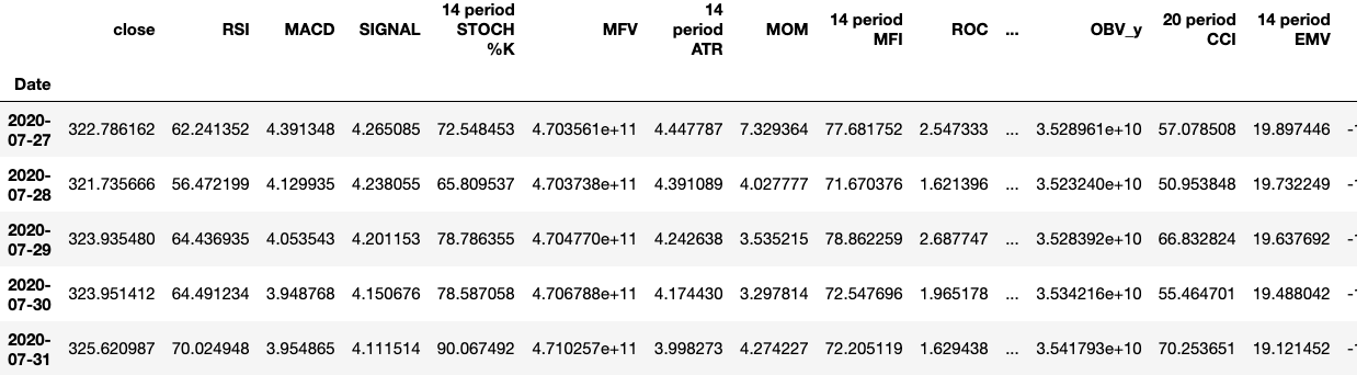

Here are the five main days we are going to generate a prediction for. Looks like the models predicts that the price will increase for each day.

这是我们要进行预测的五个主要日子。 看起来模型预测价格会每天上涨。

Lets validate our prediction with the actual results.

让我们用实际结果验证我们的预测。

del(live_pred_data['close'])prediction = ensemble_model.predict(live_pred_data)print(prediction)[1. 1. 1. 1. 1.]

Results

结果

July 27th : $ 322.78 — August 17th : $ 337.91

7月27日：$ 322.78 — 8月17日：$ 337.91

July 28th : $ 321.74 — August 18th : $ 338.64

7月28日：321.74美元-8月18日：338.64美元

July 29th : $ 323.93 — August 19th : $ 337.23

7月29日：$ 323.93 — 8月19日：$ 337.23

July 30th : $ 323.95 — August 20th : $ 338.28

7月30日：$ 323.95-8月20日：$ 338.28

July 31st : $ 325.62 — August 21st : $ 339.48

7月31日：$ 325.62-8月21日：$ 339.48

As we can see from the actual results, we can confirm that the model was correct in all of its predictions. However there are many factors that go into determining the stock price, so to say that the model will produce similar results every time is naive. However, during relatively normal periods of time (without major panic that causes volatility in the stock market), the model should be able to produce good results.

从实际结果可以看出，我们可以确认该模型在所有预测中都是正确的。 但是，决定股价的因素有很多，因此说该模型每次都会产生相似的结果是很幼稚的。 但是，在相对正常的时间段内(没有引起股票市场波动的重大恐慌)，该模型应该能够产生良好的结果。

5.总结 (5. Summary)

To summarize what we’ve done in this project,

总结一下我们在此项目中所做的工作，

1. We’ve collected data to be used in analysis and feature creation.我们已经收集了用于分析和特征创建的数据。
2. We’ve used pandas to compute many model features and produce clean data to help us in machine learning. Created predictions or truth values using pandas.我们已经使用熊猫来计算许多模型特征并生成干净的数据，以帮助我们进行机器学习。 使用熊猫创建预测或真值。
3. Trained many machine learning models and then combined them using ensemble learning to produce higher prediction accuracy.训练了许多机器学习模型，然后使用集成学习对其进行组合以产生更高的预测精度。
4. Ensured our predictions were accurate with real world data.确保我们的预测对真实世界的数据是准确的。

I’ve learned a lot about data science and machine learning through this project, and I hope you did too. Being my first article, I’d love any form of feedback to help improve my skills as a programmer and data scientist.

通过这个项目，我已经学到了很多有关数据科学和机器学习的知识，希望您也能做到。 作为我的第一篇文章，我希望获得任何形式的反馈，以帮助提高我作为程序员和数据科学家的技能。

Thanks for reading :)

谢谢阅读 ：)