R语言“优雅地“进行医学统计分析
本文首发于公众号:医学和生信笔记,完美观看体验请至公众号查看本文。
医学和生信笔记,专注R语言在临床医学中的使用,R语言数据分析和可视化。
文章目录
- 主要函数
- 描述性统计
- 比较均值
- 增强R中的ANOVA
- 事后检验(post-hoc)
- 比较比例
- 比较方差
- 计算效应量
- 相关性分析
- 计算相关性
- 重塑相关矩阵
- 相关矩阵取子集
- 可视化相关矩阵
- 添加P值和显著性标记
- 提取统计信息
- 数据处理辅助函数
- 其他
- 安装和加载
- 描述性统计
- t检验
- 单样本t检验
- 配对t检验
- 两样本t检验
- 分组后进行比较
- 多组间的两两比较
- 方差分析
- 完全随机设计方差分析
- 随机区组设计资料的方差分析
- 拉丁方设计方差分析
- 两阶段交叉设计资料方差分析
- 析因设计资料的方差分析
- 正交设计资料的方差分析
- 重复测量数据两因素两水平的方差分析
- 重复测量数据两因素多水平的分析
- 相关分析
- 两个变量
- 一个变量和其他所有变量
- 所有变量间两两相关性
- 相关矩阵
rstatix提供一个简单直观的管道友好的框架,与整洁的设计理念一致,用于执行基本的统计检验,包括t检验,Wilcoxon检验,方差分析,Kruskal-Wallis和相关性分析。每个分析的输出会自动转换成一个整洁的数据框架,以方便可视化。
附加功能可用于重塑,重新排序,操作和可视化相关矩阵。功能还包括析因实验的分析,包括重复测量设计、析因设计、正交设计等。
可以计算几个效应大小指标,包括方差分析eta平方,t检验的Cohen’s d和分类变量之间的关联的Cramer’s v。 该软件包包含用于识别单变量和多变量异常值、评估正态性和方差齐性的辅助函数。
主要函数
描述性统计
get_summary_stat():计算描述性的统计指标;freq_table(): 分类变量的频率表;get_mode(): 众数;identify_outliers(): 使用boxplot鉴别离群值;mahalanobis_distance(): 计算Mahalanobi距离和离群点;shapiro_test()andmshapiro_test(): 正态性检验.
比较均值
t_test(): 单样本、配对样本、独立样本t检验;wilcox_test(): 单样本、配对样本、独立样本秩和检验;sign_test(): 符号检验;anova_test(): 基于car::Anova()改写,可以做:独立测量、重复测量、混合anova;get_anova_test_table(): 从anova_test()提取结果,可自动执行球形检验.;welch_anova_test(): Welch one-Way ANOVA test. 基于stats::oneway.test()改写;kruskal_test(): kruskal-wallis rank sum test;friedman_test(): Friedman rank sum test;get_comparisons(): 创建需要比较的组;get_pvalue_position: 使用ggplot2添加p值时可自动计算添加坐标
增强R中的ANOVA
factorial_design(): 建立因子化的设计,方便使用car::Anova()进行分析,对于重复测量Anova非常有帮助;anova_summary(): 提取美观的Anova检验的结果,包括从car:Anova()或者stats:aov()中,主要结果包含Anova结果表、一般效应量、和一些假设检验,比如球形检验。
事后检验(post-hoc)
tukey_hsd(): tukey post-hoc tests;dunn_test(): 计算Kruskal-Wallis的成对比较;games_howell_test(): Games-Howell test;emmeans_test(): estimated marginal means
比较比例
prop_test(),pairwise_prop_test()androw_wise_prop_test(). Performs one-sample and two-samples z-test of proportions. Wrappers around the R base function prop.test() but have the advantage of performing pairwise and row-wise z-test of two proportions, the post-hoc tests following a significant chi-square test of homogeneity for 2xc and rx2 contingency tables.fisher_test(),pairwise_fisher_test()androw_wise_fisher_test(): Fisher’s exact test for count data. Wrappers around the R base function fisher.test() but have the advantage of performing pairwise and row-wise fisher tests, the post-hoc tests following a significant chi-square test of homogeneity for 2xc and rx2 contingency tables.chisq_test(),pairwise_chisq_gof_test(),pairwise_chisq_test_against_p(): Performs chi-squared tests, including goodness-of-fit, homogeneity and independence tests.binom_test(),pairwise_binom_test(),pairwise_binom_test_against_p(): Performs exact binomial test and pairwise comparisons following a significant exact multinomial test. Alternative to the chi-square test of goodness-of-fit-test when the sample.multinom_test(): performs an exact multinomial test. Alternative to the chi-square test of goodness-of-fit-test when the sample size is small.mcnemar_test(): performs McNemar chi-squared test to compare paired proportions. Provides pairwise comparisons between multiple groups.cochran_qtest(): extension of the McNemar Chi-squared test for comparing more than two paired proportions.prop_trend_test(): Performs chi-squared test for trend in proportion. This test is also known as Cochran-Armitage trend test
比较方差
levene_test(): Pipe-friendly framework to easily compute Levene’s test for homogeneity of variance across groups.box_m(): Box’s M-test for homogeneity of covariance matrices
计算效应量
cohens_d(): Compute cohen’s d measure of effect size for t-tests.wilcox_effsize(): Compute Wilcoxon effect size ®.eta_squared()andpartial_eta_squared(): Compute effect size for ANOVA.kruskal_effsize(): Compute the effect size for Kruskal-Wallis test as the eta squared based on the H-statistic.friedman_effsize(): Compute the effect size of Friedman test using the Kendall’s W value.cramer_v(): Compute Cramer’s V, which measures the strength of the association between categorical variables
相关性分析
计算相关性
cor_test(): correlation test between two or more variables using Pearson, Spearman or Kendall methods.cor_mat(): compute correlation matrix with p-values. Returns a data frame containing the matrix of the correlation coefficients. The output has an attribute named “pvalue”, which contains the matrix of the correlation test p-values.cor_get_pval(): extract a correlation matrix p-values from an object of class cor_mat().cor_pmat(): compute the correlation matrix, but returns only the p-values of the correlation tests.as_cor_mat(): convert a cor_test object into a correlation matrix format.
重塑相关矩阵
cor_reorder(): reorder correlation matrix, according to the coefficients, using the hierarchical clustering method.cor_gather(): takes a correlation matrix and collapses (or melt) it into long format data frame (paired list)cor_spread(): spread a long correlation data frame into wide format (correlation matrix).
相关矩阵取子集
cor_select(): subset a correlation matrix by selecting variables of interest.pull_triangle(),pull_upper_triangle(),pull_lower_triangle(): pull upper and lower triangular parts of a (correlation) matrix.replace_triangle(),replace_upper_triangle(),replace_lower_triangle(): replace upper and lower triangular parts of a (correlation) matrix.
可视化相关矩阵
cor_as_symbols(): replaces the correlation coefficients, in a matrix, by symbols according to the value.cor_plot(): visualize correlation matrix using base plot.cor_mark_significant(): add significance levels to a correlation matrix
添加P值和显著性标记
adjust_pvalue(): add an adjusted p-values column to a data frame containing statistical test p-valuesadd_significance(): add a column containing the p-value significance levelp_round(),p_format(),p_mark_significant(): rounding and formatting p-values
提取统计信息
get_pwc_label(): Extract label from pairwise comparisons.get_test_label(): Extract label from statistical tests.create_test_label(): Create labels from user specified test results
数据处理辅助函数
df_select(),df_arrange(),df_group_by(): wrappers arround dplyr functions for supporting standard and non standard evaluations.df_nest_by(): Nest a tibble data frame using grouping specification. Supports standard and non standard evaluations.df_split_by(): Split a data frame by groups into subsets or data panel. Very similar to the functiondf_nest_by(). The only difference is that, it adds labels to each data subset. Labels are the combination of the grouping variable levels.df_unite(): Unite multiple columns into one.df_unite_factors(): Unite factor columns. First, order factors levels then merge them into one column. The output column is a factor.df_label_both(),df_label_value(): functions to label data frames rows by by one or multiple grouping variables.df_get_var_names(): Returns user specified variable names. Supports standard and non standard evaluation
其他
doo(): alternative to dplyr::do for doing anything. Technically it usesnest()+mutate()+map()to apply arbitrary computation to a grouped data frame.sample_n_by(): sample n rows by group from a tableconvert_as_factor(),set_ref_level(),reorder_levels(): Provides pipe-friendly functions to convert simultaneously multiple variables into a factor variable.make_clean_names(): Pipe-friendly function to make syntactically valid column names (for input data frame) or names (for input vector).counts_to_cases(): converts a contingency table or a data frame of counts into a data frame of individual observations
安装和加载
if(!require(devtools)) install.packages("devtools")
devtools::install_github("kassambara/rstatix")# 或者cran
install.packages("rstatix")
加载包:
library(rstatix)
##
## 载入程辑包:'rstatix'
## The following object is masked from 'package:stats':
##
##     filter
library(ggpubr)
## 载入需要的程辑包:ggplot2
描述性统计
# 指定列
iris %>% get_summary_stats(Sepal.Length, Sepal.Width, type = "full")
## # A tibble: 2 x 13
##   variable        n   min   max median    q1    q3   iqr   mad  mean    sd    se
##   <chr>       <dbl> <dbl> <dbl>  <dbl> <dbl> <dbl> <dbl> <dbl> <dbl> <dbl> <dbl>
## 1 Sepal.Leng~   150   4.3   7.9    5.8   5.1   6.4   1.3 1.04   5.84 0.828 0.068
## 2 Sepal.Width   150   2     4.4    3     2.8   3.3   0.5 0.445  3.06 0.436 0.036
## # ... with 1 more variable: ci <dbl>
# 所有列
iris %>% get_summary_stats(type = "common")
## # A tibble: 4 x 10
##   variable         n   min   max median   iqr  mean    sd    se    ci
##   <chr>        <dbl> <dbl> <dbl>  <dbl> <dbl> <dbl> <dbl> <dbl> <dbl>
## 1 Petal.Length   150   1     6.9   4.35   3.5  3.76 1.76  0.144 0.285
## 2 Petal.Width    150   0.1   2.5   1.3    1.5  1.20 0.762 0.062 0.123
## 3 Sepal.Length   150   4.3   7.9   5.8    1.3  5.84 0.828 0.068 0.134
## 4 Sepal.Width    150   2     4.4   3      0.5  3.06 0.436 0.036 0.07
# 分组展示
iris %>% group_by(Species) %>% get_summary_stats(Sepal.Length, type = "mean_sd")
## # A tibble: 3 x 5
##   Species    variable         n  mean    sd
##   <fct>      <chr>        <dbl> <dbl> <dbl>
## 1 setosa     Sepal.Length    50  5.01 0.352
## 2 versicolor Sepal.Length    50  5.94 0.516
## 3 virginica  Sepal.Length    50  6.59 0.636
# 众数
get_mode(iris$Sepal.Length)
## [1] 5
t检验
以t检验为例。
单样本t检验
还是以之前推文中的例3-5的数据:
df <- foreign::read.spss('E:/各科资料/医学统计学/研究生课程/3总体均数的估计与假设检验18-9研/例03-05.sav',to.data.frame = T, reencode = "utf-8")
## re-encoding from utf-8attributes(df)[4] <- NULLhead(df)
##   no  hb
## 1  1 112
## 2  2 137
## 3  3 129
## 4  4 126
## 5  5  88
## 6  6  90
单样本t检验:
df %>% t_test(hb ~ 1, mu = 140)
## # A tibble: 1 x 7
##   .y.   group1 group2         n statistic    df      p
## * <chr> <chr>  <chr>      <int>     <dbl> <dbl>  <dbl>
## 1 hb    1      null model    36     -2.14    35 0.0397
结果和t.test()一样哦!
配对t检验
使用之前推文中的例3-6数据:
library(foreign)
df <- foreign::read.spss('E:/各科资料/医学统计学/研究生课程/3总体均数的估计与假设检验18-9研/例03-06.sav',to.data.frame = T, reencode = "utf-8")
## re-encoding from utf-8
attributes(df)[4] <- NULLhead(df)
##   no    x1    x2
## 1  1 0.840 0.580
## 2  2 0.591 0.509
## 3  3 0.674 0.500
## 4  4 0.632 0.316
## 5  5 0.687 0.337
## 6  6 0.978 0.517
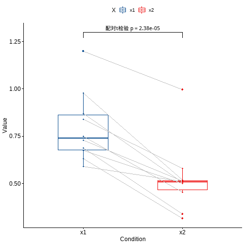
进行配对样本t检验:
library(tidyr)
st <- df %>% pivot_longer(cols = 2:3, names_to = "X", values_to = "values") %>% t_test(values ~ X, paired = T)st
## # A tibble: 1 x 8
##   .y.    group1 group2    n1    n2 statistic    df         p
## * <chr>  <chr>  <chr>  <int> <int>     <dbl> <dbl>     <dbl>
## 1 values x1     x2        10    10      7.93     9 0.0000238
结果和t.test()也是一样的哦!
可视化也可直接完成!
df %>% pivot_longer(cols = 2:3, names_to = "X", values_to = "values") %>%ggpaired(x="X",y="values",color = "X",id="no",line.size = 0.5,line.color = "grey",palette = "lancet")+stat_pvalue_manual(st,label = "配对t检验 p = {p}",y.position = 1.3)
两样本t检验
使用之前推文中的例3-8的数据
df <- foreign::read.spss('E:/各科资料/医学统计学/研究生课程/3总体均数的估计与假设检验18-9研/例03-07.sav',to.data.frame = T)
df$group <- c(rep('阿卡波糖',20),rep('拜糖平',20))
attributes(df)[3] <- NULLhead(df)
##   no    x    group
## 1  1 -0.7 阿卡波糖
## 2  2 -5.6 阿卡波糖
## 3  3  2.0 阿卡波糖
## 4  4  2.8 阿卡波糖
## 5  5  0.7 阿卡波糖
## 6  6  3.5 阿卡波糖
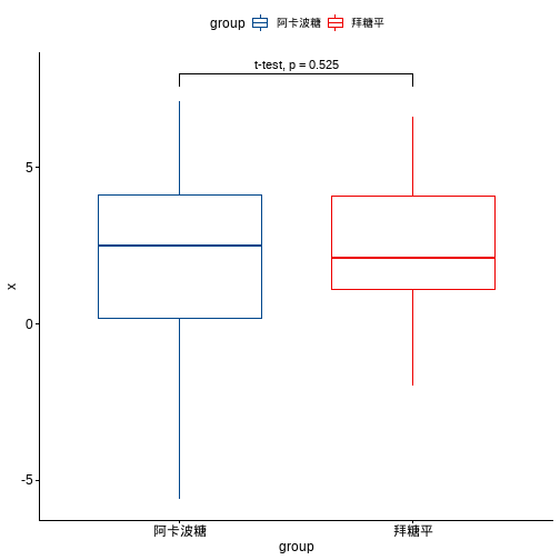
进行独立样本t检验:
dt <- df %>% t_test(x ~ group, paired = F)
dt
## # A tibble: 1 x 8
##   .y.   group1   group2    n1    n2 statistic    df     p
## * <chr> <chr>    <chr>  <int> <int>     <dbl> <dbl> <dbl>
## 1 x     阿卡波糖 拜糖平    20    20    -0.642  36.1 0.525
和自带的结果是一样的哦!
顺便可视化一起做了:
ggboxplot(df, x="group", y="x",color = "group", palette = "lancet")+stat_pvalue_manual(dt, label = "t-test, p = {p}",y.position = 8)
分组后进行比较
df <- ToothGrowth
df$dose <- as.factor(df$dose)
head(df)
##    len supp dose
## 1  4.2   VC  0.5
## 2 11.5   VC  0.5
## 3  7.3   VC  0.5
## 4  5.8   VC  0.5
## 5  6.4   VC  0.5
## 6 10.0   VC  0.5
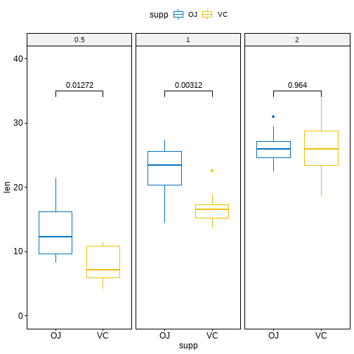
stat.test <- df %>%group_by(dose) %>%t_test(len ~ supp) %>%adjust_pvalue() %>%add_significance("p.adj")
stat.test
## # A tibble: 3 x 11
##   dose  .y.   group1 group2    n1    n2 statistic    df       p   p.adj
## * <fct> <chr> <chr>  <chr>  <int> <int>     <dbl> <dbl>   <dbl>   <dbl>
## 1 0.5   len   OJ     VC        10    10    3.17    15.0 0.00636 0.0127
## 2 1     len   OJ     VC        10    10    4.03    15.4 0.00104 0.00312
## 3 2     len   OJ     VC        10    10   -0.0461  14.0 0.964   0.964
## # ... with 1 more variable: p.adj.signif <chr>
ggboxplot(df, x = "supp", y = "len",color = "supp", palette = "jco", facet.by = "dose",ylim = c(0, 40)) +stat_pvalue_manual(stat.test, label = "p.adj", y.position = 35)
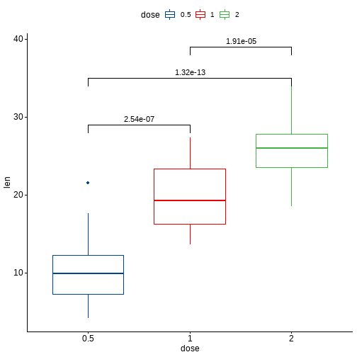
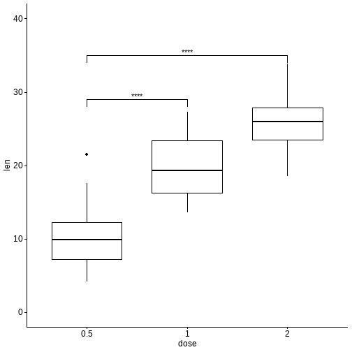
多组间的两两比较
如果有大于2个分组,会自动进行两两比较。
# 两两之间做t检验,自动完成
pairwise.test <- df %>% t_test(len ~ dose)
pairwise.test
## # A tibble: 3 x 10
##   .y.   group1 group2    n1    n2 statistic    df        p    p.adj p.adj.signif
## * <chr> <chr>  <chr>  <int> <int>     <dbl> <dbl>    <dbl>    <dbl> <chr>
## 1 len   0.5    1         20    20     -6.48  38.0 1.27e- 7 2.54e- 7 ****
## 2 len   0.5    2         20    20    -11.8   36.9 4.4 e-14 1.32e-13 ****
## 3 len   1      2         20    20     -4.90  37.1 1.91e- 5 1.91e- 5 ****
可视化:
ggboxplot(df, x = "dose", y = "len", color = "dose", palette = "lancet")+stat_pvalue_manual(pairwise.test, label = "p.adj",y.position = c(29, 35, 39))
还可以指定和某一个组进行比较:
# T-test: 都和指定的组进行比较
stat.test <- df %>% t_test(len ~ dose, ref.group = "0.5")
stat.test
## # A tibble: 2 x 10
##   .y.   group1 group2    n1    n2 statistic    df        p    p.adj p.adj.signif
## * <chr> <chr>  <chr>  <int> <int>     <dbl> <dbl>    <dbl>    <dbl> <chr>
## 1 len   0.5    1         20    20     -6.48  38.0 1.27e- 7 1.27e- 7 ****
## 2 len   0.5    2         20    20    -11.8   36.9 4.4 e-14 8.8 e-14 ****
# Box plot
ggboxplot(df, x = "dose", y = "len", ylim = c(0, 40)) +stat_pvalue_manual(stat.test, label = "p.adj.signif",y.position = c(29, 35))
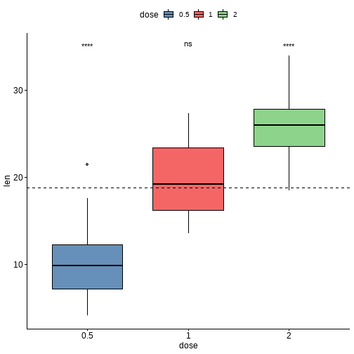
和全部数据进行比较:
stat.test <- df %>% t_test(len ~ dose, ref.group = "all")
stat.test
## # A tibble: 3 x 10
##   .y.   group1 group2    n1    n2 statistic    df           p      p.adj p.adj.signif
## * <chr> <chr>  <chr>  <int> <int>     <dbl> <dbl>       <dbl>      <dbl> <chr>
## 1 len   all    0.5       60    20     5.82   56.4 0.00000029  0.00000087 ****
## 2 len   all    1         60    20    -0.660  57.5 0.512       0.512      ns
## 3 len   all    2         60    20    -5.61   66.5 0.000000425 0.00000087 ****
ggboxplot(df, x = "dose", y = "len", fill = "dose", palette = "lancet", alpha = 0.6) +stat_pvalue_manual(stat.test, label = "p.adj.signif", y.position = 35) +geom_hline(yintercept = mean(df$len), linetype = 2)
方差分析
完全随机设计方差分析
使用课本例4-2的数据。
首先是构造数据,本次数据自己从书上摘录。。
trt<-c(rep("group1",30),rep("group2",30),rep("group3",30),rep("group4",30))weight<-c(3.53,4.59,4.34,2.66,3.59,3.13,3.30,4.04,3.53,3.56,3.85,4.07,1.37,3.93,2.33,2.98,4.00,3.55,2.64,2.56,3.50,3.25,2.96,4.30,3.52,3.93,4.19,2.96,4.16,2.59,2.42,3.36,4.32,2.34,2.68,2.95,2.36,2.56,2.52,2.27,2.98,3.72,2.65,2.22,2.90,1.98,2.63,2.86,2.93,2.17,2.72,1.56,3.11,1.81,1.77,2.80,3.57,2.97,4.02,2.31,2.86,2.28,2.39,2.28,2.48,2.28,3.48,2.42,2.41,2.66,3.29,2.70,2.66,3.68,2.65,2.66,2.32,2.61,3.64,2.58,3.65,3.21,2.23,2.32,2.68,3.04,2.81,3.02,1.97,1.68,0.89,1.06,1.08,1.27,1.63,1.89,1.31,2.51,1.88,1.41,3.19,1.92,0.94,2.11,2.81,1.98,1.74,2.16,3.37,2.97,1.69,1.19,2.17,2.28,1.72,2.47,1.02,2.52,2.10,3.71)data1<-data.frame(trt,weight)head(data1)
##      trt weight
## 1 group1   3.53
## 2 group1   4.59
## 3 group1   4.34
## 4 group1   2.66
## 5 group1   3.59
## 6 group1   3.13
进行完全随机设计资料的方差分析:
data1 %>% anova_test(weight ~ trt)
## Coefficient covariances computed by hccm()
## ANOVA Table (type II tests)
##
##   Effect DFn DFd      F        p p<.05   ges
## 1    trt   3 116 24.884 1.67e-12     * 0.392
随机区组设计资料的方差分析
使用例4-3的数据。
首先是构造数据,本次数据自己从书上摘录。。
weight <- c(0.82,0.65,0.51,0.73,0.54,0.23,0.43,0.34,0.28,0.41,0.21,0.31,0.68,0.43,0.24)
block <- c(rep(c("1","2","3","4","5"),each=3))
group <- c(rep(c("A","B","C"),5))data4_4 <- data.frame(weight,block,group)head(data4_4)
##   weight block group
## 1   0.82     1     A
## 2   0.65     1     B
## 3   0.51     1     C
## 4   0.73     2     A
## 5   0.54     2     B
## 6   0.23     2     C
数据一共3列,第一列是小白鼠肉瘤重量,第二列是区组因素(5个区组),第三列是分组(一共3组)
进行随机区组设计资料的方差分析:
data4_4 %>% anova_test(weight ~ group + block)
## Coefficient covariances computed by hccm()
## ANOVA Table (type II tests)
##
##   Effect DFn DFd      F     p p<.05   ges
## 1  group   2   8 11.937 0.004     * 0.749
## 2  block   4   8  5.978 0.016     * 0.749
拉丁方设计方差分析
使用课本例4-5的数据。
首先是构造数据,本次数据自己从书上摘录。。
psize <- c(87,75,81,75,84,66,73,81,87,85,64,79,73,73,74,78,73,77,77,68,69,74,76,73,64,64,72,76,70,81,75,77,82,61,82,61)
drug <- c("C","B","E","D","A","F","B","A","D","C","F","E","F","E","B","A","D","C","A","F","C","B","E","D","D","C","F","E","B","A","E","D","A","F","C","B")
col_block <- c(rep(1:6,6))
row_block <- c(rep(1:6,each=6))
mydata <- data.frame(psize,drug,col_block,row_block)
mydata$col_block <- factor(mydata$col_block)
mydata$row_block <- factor(mydata$row_block)
str(mydata)
## 'data.frame':  36 obs. of  4 variables:
##  $ psize    : num  87 75 81 75 84 66 73 81 87 85 ...
##  $ drug     : chr  "C" "B" "E" "D" ...
##  $ col_block: Factor w/ 6 levels "1","2","3","4",..: 1 2 3 4 5 6 1 2 3 4 ...
##  $ row_block: Factor w/ 6 levels "1","2","3","4",..: 1 1 1 1 1 1 2 2 2 2 ...
数据一共4列,第一列是皮肤疱疹大小,第二列是不同药物(处理因素,共5种),第三列是列区组因素,第四列是行区组因素。
进行拉丁方设计的方差分析:
mydata %>% anova_test(psize ~ drug + col_block + row_block)
## Coefficient covariances computed by hccm()
## ANOVA Table (type II tests)
##
##      Effect DFn DFd     F     p p<.05   ges
## 1      drug   5  20 3.906 0.012     * 0.494
## 2 col_block   5  20 0.500 0.772       0.111
## 3 row_block   5  20 1.466 0.245       0.268
两阶段交叉设计资料方差分析
使用课本例4-6的数据。
首先是构造数据,本次数据自己从书上摘录。。
contain <- c(760,770,860,855,568,602,780,800,960,958,940,952,635,650,440,450,528,530,800,803)
phase <- rep(c("phase_1","phase_2"),10)
type <- c("A","B","B","A","A","B","A","B","B","A","B","A","A","B","B","A","A","B","B","A")
testid <- rep(1:10,each=2)
mydata <- data.frame(testid,phase,type,contain)str(mydata)
## 'data.frame':  20 obs. of  4 variables:
##  $ testid : int  1 1 2 2 3 3 4 4 5 5 ...
##  $ phase  : chr  "phase_1" "phase_2" "phase_1" "phase_2" ...
##  $ type   : chr  "A" "B" "B" "A" ...
##  $ contain: num  760 770 860 855 568 602 780 800 960 958 ...mydata$testid <- factor(mydata$testid)
数据一共4列,第一列是受试者id,第二列是不同阶段,第三列是测定方法,第四列是测量值。
进行两阶段交叉设计资料方差分析:
mydata %>% anova_test(contain ~ phase + type + testid)
## Coefficient covariances computed by hccm()
## ANOVA Table (type II tests)
##
##   Effect DFn DFd        F        p p<.05   ges
## 1  phase   1   8    9.925 1.40e-02     * 0.554
## 2   type   1   8    4.019 8.00e-02       0.334
## 3 testid   9   8 1240.195 1.32e-11     * 0.999
结果和课本一致!
析因设计资料的方差分析
使用课本例11-1的数据,自己手动摘录:
df11_1 <- data.frame(x1 = rep(c("外膜缝合","束膜缝合"), each = 10),x2 = rep(c("缝合1个月","缝合2个月"), each = 5),y = c(10,10,40,50,10,30,30,70,60,30,10,20,30,50,30,50,50,70,60,30)
)str(df11_1)
## 'data.frame':  20 obs. of  3 variables:
##  $ x1: chr  "外膜缝合" "外膜缝合" "外膜缝合" "外膜缝合" ...
##  $ x2: chr  "缝合1个月" "缝合1个月" "缝合1个月" "缝合1个月" ...
##  $ y : num  10 10 40 50 10 30 30 70 60 30 ...
数据一共3列,第1列是缝合方法,第2列是时间,第3列是轴突通过率。
进行析因设计资料的方差分析:
df11_1 %>% anova_test(y ~ x1 * x2)
## Coefficient covariances computed by hccm()
## ANOVA Table (type II tests)
##
##   Effect DFn DFd     F     p p<.05   ges
## 1     x1   1  16 0.600 0.450       0.036
## 2     x2   1  16 8.067 0.012     * 0.335
## 3  x1:x2   1  16 0.067 0.800       0.004
正交设计资料的方差分析
使用课本例11-4的数据
df11_4 <- data.frame(a = rep(c("5度","25度"),each = 4),b = rep(c(0.5, 5.0), each = 2),c = c(10, 30),d = c(6.0, 8.0,8.0,6.0,8.0,6.0,6.0,8.0),x = c(86,95,91,94,91,96,83,88)
)df11_4$a <- factor(df11_4$a)
df11_4$b <- factor(df11_4$b)
df11_4$c <- factor(df11_4$c)
df11_4$d <- factor(df11_4$d)str(df11_4)
## 'data.frame':  8 obs. of  5 variables:
##  $ a: Factor w/ 2 levels "25度","5度": 2 2 2 2 1 1 1 1
##  $ b: Factor w/ 2 levels "0.5","5": 1 1 2 2 1 1 2 2
##  $ c: Factor w/ 2 levels "10","30": 1 2 1 2 1 2 1 2
##  $ d: Factor w/ 2 levels "6","8": 1 2 2 1 2 1 1 2
##  $ x: num  86 95 91 94 91 96 83 88
进行正交设计资料的方差分析:
df11_4 %>% anova_test(x ~ a + b + c + d + a * b)
## Coefficient covariances computed by hccm()
## ANOVA Table (type II tests)
##
##   Effect DFn DFd    F     p p<.05   ges
## 1      a   1   2  3.2 0.216       0.615
## 2      b   1   2  7.2 0.115       0.783
## 3      c   1   2 24.2 0.039     * 0.924
## 4      d   1   2  1.8 0.312       0.474
## 5    a:b   1   2 20.0 0.047     * 0.909
重复测量数据两因素两水平的方差分析
使用课本例12-1的数据,直接读取:
df12_1 <- foreign::read.spss("E:/各科资料/医学统计学/研究生课程/析因设计重复测量/9重复测量18-9研/12-1.sav", to.data.frame = T)str(df12_1)
## 'data.frame':  20 obs. of  5 variables:
##  $ n    : num  1 2 3 4 5 6 7 8 9 10 ...
##  $ x1   : num  130 124 136 128 122 118 116 138 126 124 ...
##  $ x2   : num  114 110 126 116 102 100 98 122 108 106 ...
##  $ group: Factor w/ 2 levels "处理组","对照组": 1 1 1 1 1 1 1 1 1 1 ...
##  $ d    : num  16 14 10 12 20 18 18 16 18 18 ...
##  - attr(*, "variable.labels")= Named chr [1:5] "编号" "治疗前血压" "治疗后血压" "组别" ...
##   ..- attr(*, "names")= chr [1:5] "n" "x1" "x2" "group" ...
##  - attr(*, "codepage")= int 936
数据一共5列(第5列是自己算出来的,其实原始数据只有4列),第1 列是编号,第2列是治疗前血压,第3例是治疗后血压,第4列是分组,第5列是血压前后差值。
进行重复测量数据两因素两水平的方差分析前,先把数据转换一下格式:
suppressMessages(library(tidyverse))
df12_11 <- df12_1[,1:4] %>% pivot_longer(cols = 2:3,names_to = "time",values_to = "hp") %>% mutate_if(is.character, as.factor)df12_11$n <- factor(df12_11$n)str(df12_11)
## tibble [40 x 4] (S3: tbl_df/tbl/data.frame)
##  $ n    : Factor w/ 20 levels "1","2","3","4",..: 1 1 2 2 3 3 4 4 5 5 ...
##  $ group: Factor w/ 2 levels "处理组","对照组": 1 1 1 1 1 1 1 1 1 1 ...
##  $ time : Factor w/ 2 levels "x1","x2": 1 2 1 2 1 2 1 2 1 2 ...
##  $ hp   : num [1:40] 130 114 124 110 136 126 128 116 122 102 ...
进行重复测量数据两因素两水平的方差分析:
hp是因变量,time是测量时间(治疗前和治疗后各测量一次),group是分组因素(两种治疗方法),n是受试者编号
df12_11 %>% anova_test(hp ~ time * group + Error(n/time))
## ANOVA Table (type II tests)
##
##       Effect DFn DFd      F        p p<.05   ges
## 1      group   1  18  1.574 2.26e-01       0.071
## 2       time   1  18 55.008 7.08e-07     * 0.278
## 3 group:time   1  18 18.771 4.01e-04     * 0.116
这个结果也是和课本一样的,只不过没有显示组内误差的情况!
重复测量数据两因素多水平的分析
使用课本例12-3的数据,直接读取:
df12_3 <- foreign::read.spss("E:/各科资料/医学统计学/研究生课程/析因设计重复测量/9重复测量18-9研/例12-03.sav",to.data.frame = T)str(df12_3)
## 'data.frame':  15 obs. of  7 variables:
##  $ No   : num  1 2 3 4 5 6 7 8 9 10 ...
##  $ group: Factor w/ 3 levels "A","B","C": 1 1 1 1 1 2 2 2 2 2 ...
##  $ t0   : num  120 118 119 121 127 121 122 128 117 118 ...
##  $ t1   : num  108 109 112 112 121 120 121 129 115 114 ...
##  $ t2   : num  112 115 119 119 127 118 119 126 111 116 ...
##  $ t3   : num  120 126 124 126 133 131 129 135 123 123 ...
##  $ t4   : num  117 123 118 120 126 137 133 142 131 133 ...
##  - attr(*, "variable.labels")= Named chr [1:7] "序号" "组别" "" "" ...
##   ..- attr(*, "names")= chr [1:7] "No" "group" "t0" "t1" ...
数据一共7列,第1列是患者编号,第2列是诱导方法(3种),第3-7列是5个时间点的血压。
首先转换数据格式:
library(tidyverse)df12_31 <- df12_3 %>% pivot_longer(cols = 3:7, names_to = "times", values_to = "hp")df12_31$No <- factor(df12_31$No)
df12_31$times <- factor(df12_31$times)str(df12_31)
## tibble [75 x 4] (S3: tbl_df/tbl/data.frame)
##  $ No   : Factor w/ 15 levels "1","2","3","4",..: 1 1 1 1 1 2 2 2 2 2 ...
##  $ group: Factor w/ 3 levels "A","B","C": 1 1 1 1 1 1 1 1 1 1 ...
##  $ times: Factor w/ 5 levels "t0","t1","t2",..: 1 2 3 4 5 1 2 3 4 5 ...
##  $ hp   : num [1:75] 120 108 112 120 117 118 109 115 126 123 ...
进行重复测量两因素多水平的方差分析:
df12_31 %>% anova_test(hp ~ times * group + Error(No/(times)))
## ANOVA Table (type II tests)
##
## $ANOVA
##        Effect DFn DFd       F        p p<.05   ges
## 1       group   2  12   5.783 1.70e-02     * 0.430
## 2       times   4  48 106.558 3.02e-23     * 0.659
## 3 group:times   8  48  19.101 1.62e-12     * 0.409
##
## $`Mauchly's Test for Sphericity`
##        Effect     W     p p<.05
## 1       times 0.293 0.178
## 2 group:times 0.293 0.178
##
## $`Sphericity Corrections`
##        Effect   GGe      DF[GG]    p[GG] p[GG]<.05   HFe      DF[HF]    p[HF]
## 1       times 0.679 2.71, 32.58 1.87e-16         * 0.896 3.59, 43.03 4.65e-21
## 2 group:times 0.679 5.43, 32.58 4.26e-09         * 0.896 7.17, 43.03 2.04e-11
##   p[HF]<.05
## 1         *
## 2         *
这个结果也是和课本一样的,而且直接给出了球形检验的结果!非常方便。
相关分析
以R语言自带的mtcars数据集为例。
mydata <- mtcars %>% select(mpg, disp, hp, drat, wt, qsec)head(mydata)
##                    mpg disp  hp drat    wt  qsec
## Mazda RX4         21.0  160 110 3.90 2.620 16.46
## Mazda RX4 Wag     21.0  160 110 3.90 2.875 17.02
## Datsun 710        22.8  108  93 3.85 2.320 18.61
## Hornet 4 Drive    21.4  258 110 3.08 3.215 19.44
## Hornet Sportabout 18.7  360 175 3.15 3.440 17.02
## Valiant           18.1  225 105 2.76 3.460 20.22
两个变量
mydata %>% cor_test(wt, mpg, method = "pearson")
## # A tibble: 1 x 8
##   var1  var2    cor statistic        p conf.low conf.high method
##   <chr> <chr> <dbl>     <dbl>    <dbl>    <dbl>     <dbl> <chr>
## 1 wt    mpg   -0.87     -9.56 1.29e-10   -0.934    -0.744 Pearson
一个变量和其他所有变量
mydata %>% cor_test(mpg, method = "pearson")
## # A tibble: 5 x 8
##   var1  var2    cor statistic        p conf.low conf.high method
##   <chr> <chr> <dbl>     <dbl>    <dbl>    <dbl>     <dbl> <chr>
## 1 mpg   disp  -0.85     -8.75 9.38e-10  -0.923     -0.708 Pearson
## 2 mpg   hp    -0.78     -6.74 1.79e- 7  -0.885     -0.586 Pearson
## 3 mpg   drat   0.68      5.10 1.78e- 5   0.436      0.832 Pearson
## 4 mpg   wt    -0.87     -9.56 1.29e-10  -0.934     -0.744 Pearson
## 5 mpg   qsec   0.42      2.53 1.71e- 2   0.0820     0.670 Pearson
所有变量间两两相关性
mydata %>% cor_test(method = "pearson")
## # A tibble: 36 x 8
##    var1  var2    cor statistic        p conf.low conf.high method
##    <chr> <chr> <dbl>     <dbl>    <dbl>    <dbl>     <dbl> <chr>
##  1 mpg   mpg    1       Inf    0          1          1     Pearson
##  2 mpg   disp  -0.85     -8.75 9.38e-10  -0.923     -0.708 Pearson
##  3 mpg   hp    -0.78     -6.74 1.79e- 7  -0.885     -0.586 Pearson
##  4 mpg   drat   0.68      5.10 1.78e- 5   0.436      0.832 Pearson
##  5 mpg   wt    -0.87     -9.56 1.29e-10  -0.934     -0.744 Pearson
##  6 mpg   qsec   0.42      2.53 1.71e- 2   0.0820     0.670 Pearson
##  7 disp  mpg   -0.85     -8.75 9.38e-10  -0.923     -0.708 Pearson
##  8 disp  disp   1       Inf    0          1          1     Pearson
##  9 disp  hp     0.79      7.08 7.14e- 8   0.611      0.893 Pearson
## 10 disp  drat  -0.71     -5.53 5.28e- 6  -0.849     -0.481 Pearson
## # ... with 26 more rows
可以看到所有的输出都是整洁格式的,而且都给出了详细的统计值。
相关矩阵
当然也提供了相关矩阵的方法。
cor.mat <- mydata %>% cor_mat()cor.mat
## # A tibble: 6 x 7
##   rowname   mpg  disp    hp   drat    wt   qsec
## * <chr>   <dbl> <dbl> <dbl>  <dbl> <dbl>  <dbl>
## 1 mpg      1    -0.85 -0.78  0.68  -0.87  0.42
## 2 disp    -0.85  1     0.79 -0.71   0.89 -0.43
## 3 hp      -0.78  0.79  1    -0.45   0.66 -0.71
## 4 drat     0.68 -0.71 -0.45  1     -0.71  0.091
## 5 wt      -0.87  0.89  0.66 -0.71   1    -0.17
## 6 qsec     0.42 -0.43 -0.71  0.091 -0.17  1
展示P值矩阵:
cor.mat %>% cor_get_pval()
## # A tibble: 6 x 7
##   rowname      mpg     disp           hp       drat        wt       qsec
##   <chr>      <dbl>    <dbl>        <dbl>      <dbl>     <dbl>      <dbl>
## 1 mpg     0        9.38e-10 0.000000179  0.0000178  1.29e- 10 0.0171
## 2 disp    9.38e-10 0        0.0000000714 0.00000528 1.22e- 11 0.0131
## 3 hp      1.79e- 7 7.14e- 8 0            0.00999    4.15e-  5 0.00000577
## 4 drat    1.78e- 5 5.28e- 6 0.00999      0          4.78e-  6 0.62
## 5 wt      1.29e-10 1.22e-11 0.0000415    0.00000478 2.27e-236 0.339
## 6 qsec    1.71e- 2 1.31e- 2 0.00000577   0.62       3.39e-  1 0
使用*代替p值:
cor.mat %>% cor_as_symbols() %>% pull_lower_triangle()
##   rowname mpg disp hp drat wt qsec
## 1     mpg
## 2    disp   *
## 3      hp   *    *
## 4    drat   +    +  .
## 5      wt   *    *  +    +
## 6    qsec   .    .  +
星号和相关性一起显示:
cor.mat %>% cor_mark_significant()
##   rowname       mpg      disp        hp      drat    wt qsec
## 1     mpg
## 2    disp -0.85****
## 3      hp -0.78****  0.79****
## 4    drat  0.68**** -0.71****   -0.45**
## 5      wt -0.87****  0.89****  0.66**** -0.71****
## 6    qsec     0.42*    -0.43* -0.71****     0.091 -0.17
简单的可视化:
cor.mat %>% cor_reorder() %>% cor_plot()
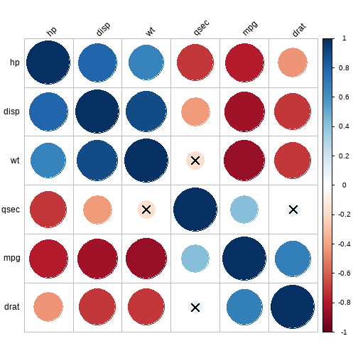
这个图明显是使用corrplot包画出来的,可以直接使用此包画出更好看的图,后期将会专门介绍corrplot包!
本文首发于公众号:医学和生信笔记,完美观看体验请至公众号查看本文。
医学和生信笔记,专注R语言在临床医学中的使用,R语言数据分析和可视化。
R语言“优雅地“进行医学统计分析相关推荐
- R语言四格表的统计分析及假设检验
R语言四格表与列联表的统计分析及假设检验 卡方检验是一种确定两个分类变量之间是否存在显着相关性的统计方法. 这两个变量应该来自相同的人口,他们应该是类似 是/否,男/女,红/绿等. 例如,我们可以建立 ...
- R:R语言实战学习一(基本统计分析)
本学期的课程R语言实战只学了前六章的皮毛,实际上后面的知识用的更多,前面的是基础,这次学习第七章:基本统计分析. 1.描述性统计分析 主要关注分析连续型变量的中心趋势.变化性和分布形状的方法,为了便于 ...
- r语言清除变量_如何优雅地计算多变量 | R语言进阶
社会科学研究经常会遇到"超多变量"的情况--多量表.多维度.多题项,以及复杂的正反计分题--如何更高效地计算量表总分?如何更简洁地进行反向计分?传统的统计工具(Excel.SPSS ...
- 在r中弄方差分析表_医学统计与R语言: qvalue
微信公众号:医学统计与R语言如果你觉得对你有帮助,欢迎转发 (FalseDiscoveryRate(FDR)=Expected(FalsePositive/(FalsePositive+TruePos ...
- 多元有序logistic回归_医学统计与R语言:多分类logistic回归HosmerLemeshow拟合优度检验...
微信公众号:医学统计与R语言如果你觉得对你有帮助,欢迎转发 输入1:multinominal logistic regression install.packages("nnet" ...
- 二元置信椭圆r语言_医学统计与R语言:圆形树状图(circular dendrogram)
微信公众号:医学统计与R语言如果你觉得对你有帮助,欢迎转发 输入1: "ggraph") 结果1: name 输入2: <- graph_from_data_frame(my ...
- 二元置信椭圆r语言_医学统计与R语言:多分类logistic回归HosmerLemeshow拟合优度检验...
微信公众号:医学统计与R语言如果你觉得对你有帮助,欢迎转发 输入1:multinominal logistic regression "nnet") 结果1: test (mult ...
- r语言library什么意思_医学统计与R语言:百分条图与雷达图
微信公众号:医学统计与R语言如果你觉得对你有帮助,欢迎转发 百分条图-输入1: library(ggplot2) 结果1: year 输入2: percentbar <- gather(perc ...
- 语言nomogram校准曲线图_医学统计与R语言:Meta 回归作图(Meta regression Plot)
微信公众号:医学统计与R语言如果你觉得对你有帮助,欢迎转发 输入1: install.packages("metafor") library(metafor) dat.bcg 结果 ...
最新文章
- windows7下java配置环境
- php$后面加点有什么用,css和js后加问号和数字有什么用
- 为什么MySQL索引更适合B+树而不是二叉树、B树
- 解决ubuntu系统udev多网卡名称变化的问题
- Spring bean注入方式
- LINUX SHELL 中if的使用
- MySQL grant 语法
- wiFI基础知识----wpa_supplicant
- Ubuntu16.04关闭笔记本触摸板
- 金蝶K3wise 演示版 W10安装
- KETTLE4个工作中有用的复杂实例--1、数据定时自动(自动抽取)同步作业
- 小程序onShareTimeline()分享朋友圈 --仅限Android
- 工具|Python常用小脚本
- YGG 联合创始人 Gabby Dizon 在 Neckerverse 峰会上分享边玩边赚的故事
- CTF-Anubis HackTheBox 渗透测试(二)
- (一)掰开了,揉碎了,说经典halcon中的那些算子
- 调试经验——使用VBA在Excel中打开Word文档(Open Word file in Excel with VBA)
- mysql命令行参数
- 大四实习生的日常(一)
- 小程序开源项目库汇总