算法组合 优化算法_算法交易简化了风险价值和投资组合优化
算法组合 优化算法
In the last post, we saw how actual algorithms are developed and tested. In this post, we will figure out the level of exposure so that can always protect our investments from significant downturns. And find the best performing portfolio given several assets.
在上一篇文章中,我们看到了如何开发和测试实际算法。 在这篇文章中,我们将弄清风险敞口水平,从而始终可以保护我们的投资免受重大衰退的影响。 并根据几种资产找到表现最佳的投资组合。
Why quantify the risk?
为什么要量化风险?
To invest or trade with confidence. Knowing Value at Risk (VaR) helps us to gauge the potential loss of equity, both in scale and frequency. Not managing this volatility can lead to significant (and avoidable) losses.
有信心地进行投资或交易。 了解风险价值(VaR)帮助我们从规模和频率上衡量潜在的股权损失。 不控制这种波动会导致重大(和可避免)的损失。
Why Optimize Portfolio?
为什么要优化投资组合?
We are all risk-averse and we want to maximize our profits. Diversification can potentially achieve both of these goals. We can select assets with the best returns that are less correlated with each other. Portfolio return and risk however depend upon final mix or weight allocation to each asset. Not getting allocation right will lead to lower returns/higher risks. We will use mean-variance optimization to find desired weights to construct the best performing portfolio(modern portfolio theory by Markowitz).
我们都规避风险,我们希望最大限度地提高利润。 多样化可以潜在地实现这两个目标。 我们可以选择相互之间关联度较低的最佳收益资产。 但是,投资组合的回报和风险取决于最终组合或对每种资产的权重分配。 分配不正确将导致较低的回报/较高的风险。 我们将使用均值方差优化来找到所需的权重,以构建表现最佳的投资组合(Markowitz的现代投资组合理论)。
Short explanation/definition of key terms
简要解释/定义关键术语
Value at Risk (VaR): Maximum dollar amount (or percentage) expected to be lost over a given time horizon, at a pre-defined confidence/probability level.
风险价值(VaR) :在给定的时间范围内,在预定义的置信度/概率水平下,预期损失的最大金额(或百分比)。
Portfolio optimization and efficient frontier: Finding best weights for selected assets such that the expected return is highest for a given risk or vice versa. An efficient frontier is simply a collection of all such dominant/optimized portfolios for all possible risk level.
投资组合优化和有效边界 :找到选定资产的最佳权重,以使给定风险的预期收益最高,反之亦然。 有效边界只是针对所有可能的风险水平的所有此类主导/优化投资组合的集合。
Sharpe ratio: Sharpe ratio is the measure of risk-adjusted return of a portfolio. Degree of excess return beyond risk-free asset for taking extra risk.
夏普比率 :夏普比率是对投资组合进行风险调整后的收益的度量。 超出无风险资产的超额收益程度,以承担额外风险。
Capital Market Line (CML): Theoretical concept that gives optimal combinations of a risk-free asset and the market portfolio (portfolio of risky assets).
资本市场线(CML) :提供无风险资产和市场投资组合(风险资产组合)的最佳组合的理论概念。
Convex optimization: Solving a mean-variance problem as convex functions, here with the help of Solvers.
凸优化 :在此处借助求解器,将均方差问题解决为凸函数。
Part 1: Value at Risk (VaR)
第1部分:风险价值(VaR)
VaR represents portfolio variance at one extreme (of the distribution). Portfolio risk is calculated as portfolio variance (equivalently standard deviation). Portfolio variance plays a major role in determining the risk characteristic of asset as a whole. Portfolio variance depends upon variance of each asset within the portfolio as well their covariance. Thus when assets are uncorrelated (do not tend to move together) portfolio risks are lower compared to portfolio of assets are highly positively correlated.
VaR代表(分布中)一种极端的投资组合方差。 投资组合风险计算为投资组合方差(等同于标准差)。 投资组合方差在确定整个资产的风险特征中起着重要作用。 投资组合方差取决于投资组合中每个资产的方差及其协方差。 因此,与不高度相关的资产组合相比,当资产不相关(不倾向于一起移动)时,资产组合的风险较低。
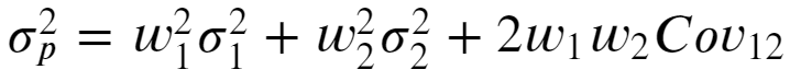
For a 2 asset portfolio, portfolio variance is given by following equation where w1, w2 are weights, sigma1, sigma2 are standard deviation of each asset and Cov12 denotes covariance between them.
对于2个资产投资组合,投资组合方差由以下等式给出,其中w1,w2是权重,sigma1,sigma2是每种资产的标准差,Cov12表示它们之间的协方差。
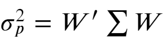
For multiple asset portfolio, position vector and covariance matrix make it much easier to express portfolio variance rather than writing a long summation.
对于多资产投资组合,位置矢量和协方差矩阵使表达投资组合方差比编写长总和变得容易得多。
Following is an expanded view of the matrix operation.
以下是矩阵运算的扩展视图。
With python (Pandas/Numpy or other tools) it is straight forward to calculate the covariance matrix for the whole asset given the series of returns. Matrix multiplication is then used to get portfolio variance.For illustration, I have taken stocks from the Nepal Stock Exchange (NEPSE). 4 highly traded stocks from different sectors were selected. The process involves loading data, calculating return for each stock, computing covariance, and finally calculating portfolio variance as given below.
使用python(Pandas / Numpy或其他工具),可以很容易地在给定一系列收益的情况下为整个资产计算协方差矩阵。 然后使用矩阵乘法获得投资组合方差。为说明起见,我从尼泊尔证券交易所(NEPSE)提取了股票。 选择了4个来自不同行业的高交易量股票。 该过程包括加载数据,计算每只股票的回报,计算协方差,最后计算投资组合方差,如下所示。
While standard deviation tells how much asset can fluctuate every day on average, VaR represents how much asset can fall a single day during a highly volatile period. VaR is expressed as a potential loss of asset (e.g. 4% of the total asset) with a certain probability (e.g. 2% chance or 98% confidence) within a certain time frame (e.g. daily/weekly). Being aware of VaR allows us to keep the right-sized asset or the right mix of assets such that we can avoid unexpected and huge losses.The image below shows that return could be as worse as or worse than -1.64 standard deviation 1 out of 20 trading days (5% probability).
标准差表示平均每天有多少资产波动,而VaR表示在高度波动的时期中一天会有多少资产下跌。 VaR表示为在特定时间范围(例如每天/每周)内具有一定概率(例如2%机会或98%的置信度)的潜在资产损失(例如总资产的4%)。 意识到VaR可以使我们保留适当大小的资产或正确的资产组合,从而避免出现意外的巨大损失。下图显示,收益可能比-1.64标准差1差或更差。 20个交易日(5%的概率)。
It is obvious that we would want a portfolio and with minimum VaR as possible for any given return. Next, we will find such a portfolio with an optimal combination of weights that has a minimum variance for a specific return. Alternatively, portfolio optimization will help us to maximize our return for any selected risk level.
显然,我们希望有一个投资组合,并且对于任何给定的回报,都需要尽可能降低VaR。 接下来,我们将找到这样的投资组合,其权重的最佳组合对于特定收益具有最小的方差。 另外,投资组合优化将帮助我们针对任何选定的风险水平最大化收益。
Example: For some random positions(weights) in 4 stocks [0.08, 0.2, 0.58, 0.14] calculated portfolio variance is 0.005, and standard deviation is 0.022 or 2.2% daily std. Assuming a normal distribution of returns, the worst 5% outcomes lie -1.64 SD away from the center. That is returns can be worse than -0.0367 or -3.67% (-1.645*0.022) in 1/20 trading days (5% chance). If we have $100000 invested, our Var at 5% probability is $3670. In other words, we tend to lose $3670 (or more) once in every 20 trading days.
例如:对于4只股票中的一些随机头寸(权重)[0.08,0.2,0.58,0.14],计算出的投资组合方差为0.005,标准差为每日std的0.022或2.2%。 假设收益呈正态分布,则最差的5%收益位于远离中心的-1.64 SD。 也就是说,在1/20个交易日内(低于5%的机会)回报可能低于-0.0367或-3.67%(-1.645 * 0.022)。 如果我们投资了100000美元,则我们以5%概率出现的Var为3670美元。 换句话说,我们倾向于每20个交易日损失3670美元(或更多)。
Part 2. Portfolio Optimization
第2部分。投资组合优化
We will gradually discover the portfolio we want in few steps. We shall start with completely random allocation (i.e. use random weights). Some of these random weight portfolios have better risk-return trade-off, hence are dominant portfolios. Those lying most upper/outer in the risk-return plot make the efficient frontier. Next, we shall find the Market portfolio by comparing the Sharpe ratio for each random portfolio. Needless to say, the Market portfolio lies on the efficient frontier and has the highest/maximum Sharpe ratio. The line tangent to this point and passing through risk-free asset is the Capital Market Line. The slope and intercept to this line are Sharpe ratio and risk-free rate respectively. Ideally, all investors select their portfolio somewhere on this line depending upon their risk/return preferences.
我们将通过几个步骤逐步发现我们想要的产品组合。 我们将从完全随机的分配开始(即使用随机权重)。 这些随机权重投资组合中的一些具有更好的风险-收益权衡 ,因此是占主导地位的投资组合 。 那些在风险收益图上位于最上/最外的人成为有效的前沿 。 接下来,我们将通过比较每个随机投资组合的夏普比率来找到市场投资组合。 不用说,市场组合位于有效的边界上,并且具有最高/最大的夏普比率。 与此切线相交并穿过无风险资产的线是资本市场线 。 这条线的斜率和截距分别是夏普比率和无风险利率。 理想情况下,所有投资者都根据风险/回报偏好选择投资组合。
A. Random allocation of weights: We will visualize the effect of random allocation weights. 1000s of portfolios are taken with random weights, respective mean and variance are calculated (and scattered for visualization). Some combination weight has better risk-return characteristics and therefore are dominating/desirable portfolios.
A.权重的随机分配:我们将可视化随机分配权重的效果。 以随机权重获取1000个投资组合,计算各自的均值和方差(并分散显示)。 一些组合权重具有更好的风险收益特性,因此是主导/理想的投资组合。
Portfolio return:
投资组合收益:
Portfolio risk:
投资组合风险:
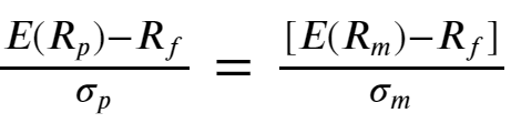
B. Market portfolio: Among all possible combinations of dominating portfolios in the efficient frontier, one which gives the highest return for taking additional risk beyond a risk-free rate is designated as a Market portfolio. we can calculate the Sharpe ratio for all portfolios given a risk-free rate and the winning portfolio with the highest Sharpe ratio is the Market Portfolio. All the rational investors gravitate towards to this best performing portfolio.This model of combining risk-free assets with the Market portfolio is known as the Capital asset pricing model (CAPM). All portfolios in CML is optimally compensated for risk above the risk-free rate. Mathematically CAPM is expressed as:
B.市场投资组合:在有效边界中所有主导投资组合的可能组合中,将承担无风险利率以外的附加风险获得最高回报的投资组合指定为市场投资组合。 在无风险利率的情况下,我们可以计算所有投资组合的夏普比率,而夏普比率最高的获胜投资组合是市场投资组合。 所有理性投资者都倾向于使用这种表现最佳的投资组合。这种将无风险资产与市场投资组合在一起的模型被称为资本资产定价模型(CAPM)。 CML中的所有投资组合都能获得高于无风险利率的最佳风险补偿。 在数学上,CAPM表示为:
Rearranging, we have Sharpe ratio for combined portfolio :
重新排列后,我们得到了组合资产组合的夏普比率:
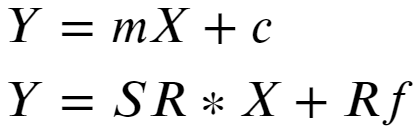
Using Rm and Sigma_m calculated from stock return and covariance Sharpe ratio for each random portfolio is calculated, one with the highest Sharpe ratio is the market/optimal portfolio.C. Capital Market Line (CML): Capital Market line represents all combinations of the risk-free asset and the optimal market portfolio. It’s easy to see that the slope of this line is the Sharpe ratio itself and the intercept is a risk-free rate. Given this information, CML can be readily drawn as seen below.
使用从股票收益率和协方差计算得出的Rm和Sigma_m,计算每个随机投资组合的Sharpe比率,夏普比率最高的是市场/最优投资组合。 资本市场线(CML):资本市场线代表无风险资产和最佳市场投资组合的所有组合。 不难看出,这条线的斜率就是夏普比率本身,截距是无风险比率。 有了这些信息,就可以很容易地绘制CML,如下所示。
Code for constructing random portfolios, finding a market portfolio, and drawing CML line.
用于构建随机投资组合,查找市场投资组合和绘制CML线的代码。
Part 3. Solvers
第3部分。求解器
Random initialization of weights can work for a portfolio with few assets but when assets grow large, the cost of computing and time it takes can be forbidding. However, solving for the best portfolio is an optimization problem with constraints. We can use Solvers from python either for getting single best return (or risk) or get the entire efficient frontier. These are solved as convex problems and the global optimum is always reached.
权重的随机初始化可以用于资产很少的投资组合,但是当资产变大时,计算成本和花费的时间可能会被禁止。 但是,求解最佳投资组合是具有约束的优化问题。 我们可以使用python的Solvers来获得单个最佳回报(或风险)或获取整个有效边界。 这些问题解决为凸问题,并且始终可以达到全局最优。
The optimization objective is expressed as:
优化目标表示为:
Here weights are represented by x and we are solving for optimal x. Objectives and constraints are written in matrix form. As a rule objective function is stated as a minimization problem. All the inequalities are similarly stated as lesser than some value.
这里的权重用x表示,我们正在求解最优x。 目标和约束以矩阵形式编写。 通常将目标函数表示为最小化问题。 类似地,所有不平等程度均小于某个值。
Inputs for Solvers:
解算器的输入:
The algorithm solves for ‘x’ with the help of inputs
该算法借助输入来求解“ x”
P or quadratic part (here it’s sigma or variance-covariance matrix, cov)
P或二次部分(此处为sigma或方差-协方差矩阵,cov)
q or linear part of the objective function (here represented by a vector of returns r or ER_stocks, above)
q或目标函数的线性部分(此处由上面的收益r或ER_stocks的向量表示)
G and h make the lower bound for weights i.e 0. We can input G as an identity matrix of size n x n (n: number of weights/stocks). Stated as matmul(G, x) < h, hence h is a vector of 0s of size n. while weights are non-negative, while solving they are stated as: -weights < 0.
G和h为权重的下限,即0。我们可以输入G作为大小为nxn的单位矩阵(n:权重/库存数)。 表示为matmul(G,x)<h,因此h是大小为n的0s的向量。 权重为非负数,而求解时权重表示为:-weights <0。
A and b make the equality part of the constraint. For our purpose the sum of all weights must equal 1. Hence A is a vector of 1s of size n. matmul(A, r_transpose) = 1, or b is simply 1.
A和b使相等性成为约束的一部分。 为了我们的目的,所有权重的总和必须等于1。因此,A是大小为n的1s的向量。 matmul(A,r_transpose)= 1或b就是1。
We can get the frontier and plot along with random portfolios:
我们可以得到边界和情节以及随机投资组合:

Code to solve using Solvers.
使用求解器求解的代码。
Limitations and Conclusion
局限性和结论
The biggest limitations of this model are the assumption of a normal distribution of returns and the validity of covariance. Actual returns are rarely normal and in fact, highly negative and positive returns are much more common giving rise to so-called fat-tailed distribution. As such the model underestimates the risks. Portfolio variance/risk is very sensitive to variance and covariance pairs i.e. the covariance matrix. Covariance rarely remains the same for a long time, hence finding a robust/valid covariance matrix is challenging.
该模型的最大局限性是假设收益呈正态分布且协方差有效。 实际收益很少是正常的,实际上,高度负收益和正收益更为普遍,从而导致所谓的肥尾分布。 因此,该模型低估了风险。 投资组合方差/风险对方差和协方差对(即协方差矩阵)非常敏感。 协方差很少会长时间保持相同,因此要找到鲁棒/有效的协方差矩阵具有挑战性。
Despite some limitations, risk modeling with VaR is a very helpful and probably most used indicator. Portfolio optimization leads to the most efficient use of our resources and any allocation decisions should be based upon these considerations. Solvers can be used to quickly find the efficient frontier or market portfolio has given return series for each stock.
尽管有一些限制,但使用VaR进行风险建模是一个非常有用且可能是最常用的指标。 投资组合优化可最有效地利用我们的资源,任何分配决策均应基于这些考虑。 解算器可用于快速找到有效的前沿或市场投资组合,从而为每只股票提供收益系列。
You can read the earlier post here:
您可以在此处阅读之前的文章:
翻译自: https://medium.com/@mnshonco/algorithmic-trading-simplified-value-at-risk-and-portfolio-optimization-ce8f0977d09
算法组合 优化算法
http://www.taodudu.cc/news/show-995245.html
相关文章:
- covid 19如何重塑美国科技公司的工作文化
- 蒙特卡洛模拟预测股票_使用蒙特卡洛模拟来预测极端天气事件
- 微生物 研究_微生物监测如何工作,为何如此重要
- web数据交互_通过体育运动使用定制的交互式Web应用程序数据科学探索任何数据...
- 熊猫数据集_用熊猫掌握数据聚合
- 数据创造价值_展示数据并创造价值
- 北方工业大学gpa计算_北方大学联盟仓库的探索性分析
- missforest_missforest最佳丢失数据插补算法
- 数据可视化工具_数据可视化
- 使用python和pandas进行同类群组分析
- 敏捷数据科学pdf_敏捷数据科学数据科学可以并且应该是敏捷的
- api地理编码_通过地理编码API使您的数据更有意义
- 分布分析和分组分析_如何通过群组分析对用户进行分组并获得可行的见解
- 数据科学家 数据工程师_数据科学家应该对数据进行版本控制的4个理由
- 数据可视化 信息可视化_可视化数据以帮助清理数据
- 使用python pandas dataframe学习数据分析
- 前端绘制绘制图表_绘制我的文学风景
- 回归分析检验_回归分析
- 数据科学与大数据技术的案例_主数据科学案例研究,招聘经理的观点
- cad2016珊瑚_预测有马的硬珊瑚覆盖率
- 用python进行营销分析_用python进行covid 19分析
- 请不要更多的基本情节
- 机器学习解决什么问题_机器学习帮助解决水危机
- 网络浏览器如何工作
- 案例与案例之间的非常规排版
- 隐私策略_隐私图标
- figma 安装插件_彩色滤光片Figma插件,用于色盲
- 设计师的10种范式转变
- 实验心得_大肠杆菌原核表达实验心得(上篇)
- googleearthpro打开没有地球_嫦娥五号成功着陆地球!为何嫦娥五号返回时会燃烧,升空却不会?...
算法组合 优化算法_算法交易简化了风险价值和投资组合优化相关推荐
- 算法偏见是什么_算法可能会使任何人(包括您)有偏见
算法偏见是什么 在上一篇文章中,我们展示了当数据将情绪从动作中剥离时会发生什么 (In the last article, we showed what happens when data strip ...
- 如何使用Python+Django+Mysql开发特色美食推荐系统 个性化美食推荐网站 个性化推荐算法开发 基于用户、物品的协同过滤推荐算法 组合、混合推荐算法FoodRecommendSystem
如何使用Python+Django+Mysql开发特色美食推荐系统 个性化美食推荐网站 个性化推荐算法开发 基于用户.物品的协同过滤推荐算法 组合.混合推荐算法FoodRecommendSystem ...
- 项目简单实用方式_组合替代继承_算法切换
算法切换 关键字:算法切换 意图: 关注算法的封装:将每一个算法封装到单独的类,使他们可以相互替换. 优点:对象(员工)与算法(岗位薪资计算方式)隔离. 缺点:客户端代码必须知道所有算法的实现,并自行 ...
- 程振波 算法设计与分析_算法设计与分析
本书按照教育部*制定的计算机科学与技术专业规范的教学大纲编写,努力与国际计算机学科的教学要求接轨.强调 算法 与 数据结构 之间密不可分的联系,因而强调融数据类型与定义在该类型上的运算于一体的抽象数据 ...
- python 算法设计与分析_算法设计与分析(黄建军)
spContent=本课基于主讲教师在北京大学讲授数据结构与算法课(Python版)的多年教学实践经验,面向具有Python语言程序设计基础的大学生和社会公众,介绍常见的基本数据结构以及相关经典算法, ...
- python分位数回归模型_如何理解分位数回归风险价值 (VaR) 模型?
风险价值(下称VaR)的计算方法主要有历史模拟法(非参数法).分析方法.蒙特-卡罗模拟法三类.不同的计算方法.计算参数下所得的VaR都是不同的.若某机构宣称其产品的VaR较低即投资风险较低,投资者还需 ...
- python中算法是指什么_算法(Python)
算法就是为了解决某一个问题而采取的具体有效的操作步骤 算法的复杂度,表示代码的运行效率,用一个大写的O加括号来表示,比如O(1),O(n) 认为算法的复杂度是渐进的,即对于一个大小为n的输入,如果他的 ...
- 算法设计与分析_算法设计与分析(第2版)第2章分治策略回顾
YI时间|外刊|MM-DFW|机器学习系列 点击上方蓝字,关注给你写干货的松子茶 分治策略是通用算法设计技术之一,很多有效的算法是它的特殊实现,顾名思义就是分而治之.一个问题能够用分治法求解的要素是 ...
- 贪心算法解决跳马问题_算法浅谈——怪盗基德的珠宝选择问题与贪心算法
点击上方蓝字,和我一起学技术. 1 在开始今天的文章之前,我们先来讲一个故事: 在一个月黑风高的夜晚,怪盗基德潜入了一个著名的珠宝会馆.他面前有三个装着珠宝的柜子,这三个规则分别是A.B和C. ...
最新文章
- Apollo 5.0,GitHub热榜第四
- 网上教育能改变教育不公平的现状吗?
- ABAP function group和Tomcat library重复加载问题
- spring依赖注入_Spring依赖注入技术的发展
- ASP.NET MVC 4 (六) 帮助函数
- (140)FPGA面试题-FPGA IP简介
- ISO 审批通过 Ada 2012 语言标准
- 浙江理工考研c语言程序设计,浙江理工大学C程序设计期末试卷A卷
- WebSocket入门使用教程
- 汽车行业与 Telematics
- (毕业设计资料)基于单片机51单片机智能药盒控制系统设计
- Footprint Analytics: 从多个维度带你进入 GameFi 领域
- ps-通道实现故障色彩效果
- 3060ti适配的cuda和cudnn
- 小码哥学习感想第一天
- 惠普暗影精灵8 Pro酷睿版和锐龙版的区别 哪个更值得入手
- 这可能是全网最全的车载OS整理
- 解读《花木兰》中的木兰形象
- gsva gsea ssgsea gaochao 使用GSVA方法计算某基因集在各个样本的表现
- 使用JS判断用户操作系统是否安装某字体