Regression with ARIMA errors combines two powerful statistical models namely, Linear Regression, and ARIMA (or Seasonal ARIMA), into a single super-powerful regression model for forecasting time series data.

具有ARIMA错误的回归将两个强大的统计模型(线性回归和ARIMA(或季节性ARIMA))组合到一个用于预测时间序列数据的超强大回归模型中。

The following schematic illustrates how Linear Regression, ARIMA and Seasonal ARIMA models are combined to produce the Regression with ARIMA errors model:

以下示意图说明了如何将线性回归，ARIMA和季节性ARIMA模型组合在一起以产生带有ARIMA误差的回归模型：

In this article, we’ll look at the most general of these models, called as Regression with Seasonal ARIMA errors or SARIMAX for short.

在本文中，我们将研究这些模型中最笼统的模型，称为季节性季节性ARIMA错误或SARIMAX的回归 。

SARIMAX —概念 (SARIMAX — the concept)

Suppose your time series data set consists of a response variable and some regression variables. Suppose also that the regression variables are contained in a matrix X, and the response variable a.k.a. dependent variable is contained in a vector y. At each time step i, y takes some value y_i and there is a corresponding row vector x_i in X containing the values of all the regression variables at time step i. This situation is illustrated by the following figure:

假设您的时间序列数据集由一个响应变量和一些回归变量组成。 还假设回归变量包含在矩阵X中 ，响应变量又称为因变量包含在向量y中 。 在每个时间步长i ， y取某个值y_i，并且X中存在一个相应的行向量x_i ，其中包含时间步长i上所有回归变量的值。 下图说明了这种情况：

A naive approach to model this data using a linear regression model as follows:

使用线性回归模型对数据进行建模的幼稚方法如下：

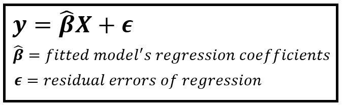
In the above model specification, β(cap) is an (m x 1) size vector storing the fitted model’s regression coefficients.

在上述模型规范中， β(cap)是一个大小为(mx 1)的向量，用于存储拟合模型的回归系数。

ε, the residual errors of regression is the difference between the actual y and the value y(cap) predicted by the model. So at each time step i: ε_i = y_i — y(cap)_i. ε is a vector of size (n x 1), assuming a data set spanning n time steps.

ε ，回归的残差是实际y与模型预测的值y(cap)之差。 因此，在每个时间步长i： ε_i= y_i — y(cap)_i。 ε 是一个大小为(nx 1)的向量，假设数据集跨越n个时间步长。

But alas, our elegant Linear Regression model will not work for time series data for a very simple reason: time series data are auto i.e. self correlated. A given value of y_i in y is influenced by previous values of y i.e. y_(i-1), y_(i-2) etc. Linear regression models are unable to ‘explain’ such auto-correlations.

但是，a，我们的优雅线性回归模型不适用于时间序列数据，原因很简单：时间序列数据是自动的，即自相关的。 Y_I的在y一个给定值由y即Y_(I-1)，Y_(I-2)等的线性回归模型无法“解释”这样自相关的先前的值的影响。

Therefore, if you fit a straight-up linear regression model to the (y, X) data set, these auto-correlations will leak into the the residual errors of regression (ε), making the ε auto-correlated!

因此，如果您将线性线性回归模型拟合为( y，X )数据集，则这些自相关将泄漏到回归的残差误差( ε )中，从而使ε自相关！

We have seen in my article on the Assumptions of Linear Regression that Linear Regression models assume that the residual errors of regression are independent random variables with identical normal distributions. But if the residual errors are auto-correlated, they cannot be independent, causing many problems. A major problem caused by auto-correlated residual errors is that one cannot use statistical tests of significance such as the F-test or the Student’s t-test to determine whether the regression coefficients are significant. Neither can one rely on the standard errors of the regression coefficients. This in turn makes the confidence intervals of the regression coefficients, and those of the model’s forecasts, unreliable. Just this one problem of auto-correlation in the residual errors, causes a cascading litany of problems with the Linear Regression model, rendering it practically useless for modeling time series data.

我们在关于线性回归假设的文章中看到，线性回归模型假设回归的残差误差是具有相同正态分布的独立随机变量。 但是，如果残差错误是自动相关的，它们就不可能独立，从而导致许多问题。 自相关残差导致的一个主要问题是，不能使用显着性统计检验(例如F检验或Student t检验)来确定回归系数是否显着。 也不能依靠回归系数的标准误差。 反过来，这会使回归系数的置信区间以及模型预测的置信区间不可靠。 残差误差中的这一自相关问题会导致线性回归模型的问题一连串出现，从而使其实际上对建模时间序列数据毫无用处。

But instead of throwing away the powerful Linear Regression model, one can fix the problem of auto-correlated residuals by bringing in another powerful model, namely ARIMA (or Seasonal ARIMA). (S)ARIMA models are perfectly suited for dealing with auto-correlated data. We harness this ability of SARIMA, by modeling the residual errors of linear regression using the SARIMA model.

但是，可以抛弃强大的线性回归模型，而可以引入另一种强大的模型ARIMA(或季节性ARIMA)来解决自相关残差的问题。 (S)ARIMA模型非常适合处理自动相关数据。 通过使用SARIMA模型对线性回归的残差建模，我们利用了SARIMA的这种能力。

SARIMA模型 (The SARIMA model)

A SARIMA model consists of the following 7 components:

SARIMA模型由以下7个组件组成：

AR: The Auto-Regressive (AR) component is a linear combination of past values of the time series up to some number of lags p. i.e. y_i is a linear combination of y_(i-1), y_(i-2),…y_(i-p) as follows:

AR：自回归(AR)组件是时间序列的过去值直至一定数量的滞后p的线性组合。 即y_i是y_(i-1) ， y_(i-2) ，… y_(ip)的线性组合，如下所示：

y_i is the actual value observed at the ith time step. The phi(cap)_i are the fitted model’s regression coefficients. The ε_i is the residual error of regression for the ith time step. The order ‘p’ of the AR(p) model is determined using a combination of well-known rules and modeler’s judgement.

y_i是在第i个时间步长处观察到的实际值。 phi(cap)_i是拟合模型的回归系数。 ε_i是第i个时间步长的回归残差。 AR(p)模型的阶次“ p”是使用众所周知的规则和建模者的判断确定的。

MA: The Moving Average (MA) component of SARIMA is a linear combination of the model’s past errors up to some number of lags q. The model’s past errors are calculated by subtracting the past predictions from past actual values. The MA(q) model is expressed as follows:

MA： SARIMA的移动平均(MA)组件是模型的过去误差直至一定数量的滞后q的线性组合。 通过从过去的实际值中减去过去的预测来计算模型的过去的误差。 MA(q)模型表示如下：

y_i is the actual value observed at the ith time step. The theta(cap)_i are the fitted model’s regression coefficients. The ε_i is the residual error of regression for the ith time step. The negative signs are as per the convention for specifying MA models. The order ‘q’ of the MA(q) model is determined using a combination of well-known rules and the modeler’s judgement.

y_i是在第i个时间步长处观察到的实际值。 theta(cap)_i是拟合模型的回归系数。 ε_i是第i个时间步长的回归残差。 负号符合指定MA模型的惯例。 MA(q)模型的阶数“ q”是使用众所周知的规则和建模者的判断确定的。

The combined ARMA (p,q) model is simply the combination of the AR(p) and MA(q) models:

组合的ARMA(p，q)模型只是AR(p)和MA(q)模型的组合：

Order of differencing (d): The ARMA model cannot be used if the time series has a trend. Common examples of trend are linear trend, quadratic trend and exponential or logarithmic trends. If the time series demonstrates a trend, one applies one or more orders of differencing to the time series so as to remove the trend. A first order difference will remove a linear trend of the type y = m*x + x. Second and higher order differences will remove polynomial trends of the kind y = m*x² + c, y = x*x³ + c etc.

差异顺序(d)：如果时间序列具有趋势，则不能使用ARMA模型。 趋势的常见示例是线性趋势，二次趋势以及指数或对数趋势。 如果时间序列显示趋势，则可以对时间序列应用一个或多个差分阶数以消除趋势。 一阶差将消除类型为y = m * x + x的线性趋势。 二阶和更高阶的差将消除类型为y = m *x²+ c ， y = x *x³+ c等的多项式趋势。

The difference operation in ARIMA models is denoted by the I letter. In ARIMA, I stands for Integrated. Differencing is applied by ARIMA models before the AR and the MA terms are brought into play. The order of differencing is denoted by the d parameter in the ARIMA(p,d,q) model specification.

ARIMA模型中的差异运算用I表示 信。 在ARIMA， 我代表我 ntegrated。 在AR和MA术语生效之前 ，ARIMA模型会应用差异。 差异的顺序由ARIMA(p，d，q)模型规范中的d参数表示。

SAR, SMA, D and m: The Seasonal ARIMA or SARIMA model simply extends the above concepts concepts of AR, MA and differencing to the seasonal realm by introducing a Seasonal AR (SAR) term of order P, Seasonal MA (SMA) term of order Q, and a Seasonal Difference of order D. The final parameter in SARIMA models is ‘m’ which is the seasonal period. For e.g. m=12 months for a time series that exhibits yearly seasonality. Just as with p,d and q, there are well established rules for estimating the values of P, D, Q and m.

SAR，SMA，D和m：季节性ARIMA或SARIMA模型通过引入P的季节性AR(SAR)项，P的季节性MA(SMA)项，将AR，MA的上述概念概念简单地扩展到季节性领域。 Q阶和D阶的季节差异。SARIMA模型中的最终参数是“ m”，它是季节周期。 例如，对于表现出年度季节性的时间序列，m = 12个月。 就像p，d和q一样，有完善的规则可以估算P，D，Q和m的值。

The complete SARIMA model specification is ARIMA(p,d,q)(P,D,Q)m.

完整的SARIMA模型规格为ARIMA(p，d，q)(P，D，Q)m。

Now let’s return to our little conundrum about auto-correlated residuals.

现在让我们回到有关自动相关残差的小难题。

As mentioned earlier, (S)ARIMA models are perfectly suited for forecasting time series data, and particularly for dealing with auto-correlated data. We apply this property of SARIMA models to model the auto-correlated residuals of the Linear Regression model after it is fitted to the time series data set.

如前所述，(S)ARIMA模型非常适合预测时间序列数据，尤其是处理自动相关数据。 在将线性回归模型拟合到时间序列数据集之后，我们将SARIMA模型的此属性用于对线性回归模型的自相关残差建模。

The resulting model is known as Regression with Seasonal ARIMA Errors or SARIMAX for short. It can be loosely specified as follows:

所得模型称为季节性ARIMA错误回归或简称为SARIMAX 。 可以宽松地指定如下：

If (p,d,q), (P,D,Q) and m are chosen correctly, one would expect the residual errors of the SARIMAX model to be not auto-correlated. In fact, they would be expected to be independent, identically distributed random variables with zero mean and some constant variance.

如果正确选择了(p，d，q)，(P，D，Q)和m，则可以预期SARIMAX模型的残留误差不会自相关。 实际上，可以预期它们是独立的，均匀分布的随机变量，具有零均值和一些恒定方差。

In this article, I will not go into the details of the rules for estimating p,d,q,P,D,Q and m. Instead, we’ll focus on building a SARIMAX model for a real world data set using Python and Statsmodels. As we go along, we’ll apply various rules for fixing SARIMAX’s parameters.

在本文中，我不会详细介绍估计p，d，q，P，D，Q和m的规则。 相反，我们将专注于使用Python和Statsmodels为现实世界的数据集构建SARIMAX模型。 在进行过程中，我们将应用各种规则来修复SARIMAX的参数。

To get a good understanding of what the full set of rules is, please refer to the following excellent link on the topic:

为了全面了解什么是完整规则，请参考以下有关该主题的出色链接：

Be sure to also review the rest of Prof. Nau’s lecture notes on ARIMA for an in-depth understanding of ARIMA and SARIMA models:

一定还要阅读Nau教授关于ARIMA的讲义的其余部分，以深入了解ARIMA和SARIMA模型：

使用Python和statsmodels建立具有季节性ARIMA错误的回归模型 (Using Python and statsmodels to build a Regression model with Seasonal ARIMA errors)

We’ll put to use what we’ve learned so far. We’ll design a SARIMAX model for a real world data set. The data set we’ll use contains hourly readings of various air pollutants measured at a busy intersection in an Italian city from 2004 to 2005. Here’s the link to the original data set:

我们将使用到目前为止所学的知识。 我们将为现实世界的数据集设计一个SARIMAX模型。 我们将使用的数据集包含从2004年到2005年在意大利城市繁忙的十字路口测量的各种空气污染物的每小时读数。这是原始数据集的链接：

https://archive.ics.uci.edu/ml/datasets/Air+quality

https://archive.ics.uci.edu/ml/datasets/Air+quality

I have adapted this data set for our SARIMAX experiment. The modified data set can be downloaded from here.

我已将此数据集用于我们的SARIMAX实验。 可以从此处下载修改后的数据集。

Let’s begin by importing all the Python packages we will be using:

首先导入所有将要使用的Python软件包：

import pandas as pdfrom statsmodels.regression import linear_modelfrom patsy import dmatricesimport statsmodels.graphics.tsaplots as tsafrom matplotlib import pyplot as pltfrom statsmodels.tsa.seasonal import seasonal_decomposefrom statsmodels.tsa.arima.model import ARIMA as ARIMAimport numpy as np

We’ll use pandas to load the data into a DataFrame:

我们将使用pandas将数据加载到DataFrame中：

df = pd.read_csv('air_quality_uci.csv', header=0)

Let’s print out the first 10 rows:

让我们打印出前10行：

df.head(10)

回归目标 (Regression Goal)

We’ll build a regression model to predict the hourly value of the PT08_S4_NO2 variable.

我们将建立一个回归模型来预测PT08_S4_NO2变量的小时值。

回归策略 (Regression strategy)

Our model’s variables will be as follows:

我们模型的变量如下：

Dependent variable y is PT08_S4_NO2

因变量y为PT08_S4_NO2

The matrix of regression variables X will contain two variables:Temperature TAbsolute Humidity AH

回归变量X的矩阵将包含两个变量：温度T绝对湿度AH

We will use the Regression with (Seasonal) ARIMA errors i.e. the (S)ARIMAX model to predict hourly values of PT08_S4_NO2 using hourly measurements of Temperature and Absolute Humidity.

我们将使用具有(季节性)ARIMA错误的回归，即(S)ARIMAX模型，使用每小时的温度和绝对湿度测量来预测PT08_S4_NO2的每小时值。

Since we are using (S)ARIMAX, we may also implicitly use past values of the dependent variable PT08_S4_NO2 and past errors of the model as additional regression variables.

由于我们使用的是(S)ARIMAX，因此我们也可以隐式使用因变量PT08_S4_NO2的过去值和模型的过去误差作为附加回归变量。

I have put (Seasonal) or (S) in brackets for now, since we don’t yet know whether there is any seasonality present in the residual errors of the regression. We’ll find that out soon enough.

我现在将(Seasonal)或(S)放在方括号中，因为我们尚不知道回归的残留误差中是否存在任何季节性。 我们会尽快发现这一点。

We’ll use the following step-by-step procedure to build the (S)ARIMAX model:

我们将使用以下分步过程来构建(S)ARIMAX模型：

步骤1：准备数据 (STEP 1: Prepare the data)

Convert the dateTime column in the data frame into a pandas DateTime column and set it as the index of the DataFrame.

将数据框中的dateTime列转换为pandas DateTime列，并将其设置为DataFrame的索引。

df['DateTimeIndex']= pd.to_datetime(df['DateTime'])df = df.set_index(keys=['DateTimeIndex'])

Set the frequency attribute of the index to Hourly. This will create several empty rows corresponding to the missing hourly measurements in the original data set. Fill up all the empty data cells with the mean of the corresponding column.

将索引的频率属性设置为每小时。 这将创建几个与原始数据集中缺少的每小时测量值相对应的空行。 用相应列的平均值填充所有空数据单元格。

df = df.asfreq('H')df = df.fillna(df.mean())

Verify that there are no empty cells in any column. The output should be all zeroes.

验证任何列中没有空单元格。 输出应全为零。

df.isin([np.nan, np.inf, -np.inf]).sum()

Create the training and the test data sets. Set the test data set length to be 10% of the training data set. We won’t actually need it to be that big, but let’s go with 10% for now.

创建培训和测试数据集。 将测试数据集的长度设置为训练数据集的10％。 我们实际上并不需要它那么大，但是现在让我们考虑10％。

dataset_len = len(df)split_index = round(dataset_len*0.9)train_set_end_date = df.index[split_index]df_train = df.loc[df.index <= train_set_end_date].copy()df_test = df.loc[df.index > train_set_end_date].copy()

步骤2：建立线性回归模型 (STEP 2: Create a Linear Regression model)

We’ll now fit an Ordinary Least Squares Linear Regression model on the training data set and fetch it’s vector of residual errors.

现在，我们在训练数据集上拟合普通最小二乘线性回归模型，并获取其为残差向量。

Let’s create the model expression in Patsy syntax. In the expression below, we are saying that PT08_S4_NO2 is the dependent variable and T and AH are the regression variables. An intercept term is assumed by default.

让我们以Patsy语法创建模型表达式。 在下面的表达式中，我们说PT08_S4_NO2是因变量，而T和AH是回归变量。 默认情况下采用拦截项。

expr = 'PT08_S4_NO2 ~ T + AH'

Let’s carve out the y and X matrices. Patsy makes this really simple:

让我们找出y和X矩阵。 Patsy使这变得非常简单：

y_train, X_train = dmatrices(expr, df_train, return_type='dataframe')y_test, X_test = dmatrices(expr, df_test, return_type='dataframe')

Fit an OLSR model on the training dataset:

在训练数据集上拟合OLSR模型：

olsr_results = linear_model.OLS(y_train, X_train).fit()

Print out the OLSR model’s training results:

打印OLSR模型的训练结果：

olsr_results.summary()

We see the following output. I have highlighted a couple of significant areas in the output:

我们看到以下输出。 我在输出中突出了几个重要方面：

We see that the regression coefficients of both regression variables T and AH are significant at a 99.99% confidence level as indicated by their P values (P > |t| column) which are essentially 0.

我们看到，回归变量T和AH的回归系数在99.99％的置信度上均很显着，如其P值(P> | t |列)所表示的，该值基本上为0。

The second thing to note in these results is the output of the Durbin-Watson test which measures the degree of LAG-1 auto-correlation in the residual errors of regression. A value of 2 implies no LAG-1 auto-correlation. A value closer to 0 implies strong positive auto-correlation while a value close to 4 implies a strong negative auto-correlation at LAG-1 among the residuals errors ε.

这些结果中要注意的第二件事是Durbin-Watson检验的输出，该检验测量回归残差中LAG-1自相关的程度。 值2表示没有LAG-1自相关。 接近0的值表示残差误差ε中的LAG-1处的强正自相关，而接近4的值则隐含强的自相关。

In the above output, we see that the DW test statistic is 0.348 indicating a strong positive auto-correlation among the residual errors of regression at LAG-1. This was completely expected since the underlying data is a time series and the linear regression model has failed to explain the auto-correlation in the dependent variable. The DW test statistic just confirms it.

在上面的输出中，我们看到DW检验统计量为0.348，表明在LAG-1处的回归残留误差之间有很强的正自相关。 这完全可以预期，因为基础数据是时间序列，并且线性回归模型无法解释因变量的自相关。 DW测试统计信息只是对其进行确认。

步骤3：估算(S)ARIMA参数(p，d，q)，(P，D，Q)和m (STEP 3: Estimate (S)ARIMA parameters (p,d,q), (P,D,Q) and m)

We now begin the process of estimating the parameters of the SARIMA model on the OLSR model’s residual errors of regression ε. The regression errors are stored in the variable olsr_results.resid.

现在我们开始在OLSR模型的回归ε残差上估计SARIMA模型的参数的过程。 回归误差 存储在变量olsr_results.resid 。

Let’s start with plotting the Auto-correlation plot of the residual errors:

让我们从绘制残差的自相关图开始：

tsa.plot_acf(olsr_results.resid, alpha=0.05)plt.show()

We get the following plot:

我们得到以下图：

The ACF tells us three things:

ACF告诉我们三件事：

1. There are strong auto-correlations extending out to multiple lags indicating that the residual errors time series has a trend. We’ll need to de-trend this time series by using one or possibly 2 orders of differencing. Thus, the parameter d is likely to be 1, or possibly 2.

   有很强的自相关性延伸到多个滞后，表明残余误差时间序列具有趋势。 我们需要通过使用一阶或二阶微分来消除这个时间序列的趋势。 因此，参数d可能为1，或者可能为2。

2. The wavelike pattern in the ACF evidences a seasonal variation in the data.

   ACF中的波形模式表明了数据的季节性变化。

3. The peak at LAG = 24 indicates that the seasonal period is likely to be 24 hours. i.e. m is likely to be 24. This seems reasonable for data containing vehicular pollution measurements. We’ll soon verify this guess using the time series decomposition plot.

   LAG = 24的峰值表明该季节可能是24小时。 即m可能是24 。 对于包含车辆污染测量值的数据，这似乎是合理的。 我们将很快使用时间序列分解图来验证这一猜测。

Quick note: the LAG-0 autocorrelation will always be a perfect 1.0 and can be ignored as a value is perfectly correlated with itself.

快速说明：LAG-0自相关将始终是完美的1.0，并且可以忽略，因为值与自身完美相关。

Before we estimate the rest of the (S)ARIMA parameters, let’s difference the time series once i.e. d=1:

在估算其余(S)ARIMA参数之前，让我们对时间序列进行一次差分，即d = 1：

olsr_resid_diff_1 = olsr_results.resid.diff()olsr_resid_diff_1 = olsr_resid_diff_1.dropna()

Let’s replot the ACF of the differenced time series of residual errors:

让我们重新绘制残差不同时间序列的ACF：

tsa.plot_acf(olsr_resid_diff_1, alpha=0.05)plt.show()

We now see a very different picture in the ACF. The auto-correlations are significantly reduced at all lags. The wavelike pattern still exists but that’s because we did nothing to remove the possible seasonal variation. The LAG-24 auto-correlation is once again especially prominent.

现在，我们在ACF中看到了完全不同的图片。 在所有滞后，自相关都显着降低。 波动模式仍然存在，但这是因为我们没有采取任何措施消除可能的季节性变化。 LAG-24自相关再次特别突出。

We see that there is still a significant auto-correlation at LAG-1 in the differenced time series. We could try extinguishing it by taking one more difference, i.e. d=2 and plotting the resulting time series’ ACF:

我们看到，在不同的时间序列中，LAG-1仍存在显着的自相关。 我们可以尝试通过再减去一个差即d = 2并绘制结果时间序列的ACF 来消除它：

olsr_resid_diff_2 = olsr_resid_diff_1.diff()olsr_resid_diff_2 = olsr_resid_diff_2.dropna()tsa.plot_acf(olsr_resid_diff_2, alpha=0.05)plt.show()

We get the following plot:

我们得到以下图：

Unfortunately, diff-ing the time series a second time has produced a heavy negative auto-correlation at LAG-1. This is bad sign. We seem to have over-done the differencing. We should stick with d=1.

不幸的是，第二次比较时间序列在LAG-1处产生了严重的负自相关。 这是坏兆头。 我们似乎对差异做得过大。 我们应该坚持d = 1。

Let’s revisit the ACF of the DIFF(1) time series:

让我们回顾一下DIFF(1)时间序列的ACF：

The single positive auto-correlation at LAG-1 indicates that we may want to fix the AR order p to 1. i.e. an AR(1) model.

LAG-1处的单个正自相关表明我们可能希望将AR阶p固定为1，即AR(1)模型 。

Since we have fixed p to 1, for now, we’ll leave out the MA portion of the model. i.e. we fix q to 0. i.e. our SARIMA model will not have an MA component.

由于我们现在将p固定为1，因此我们将省略模型的MA部分。 即我们将q固定为0。即我们的SARIMA模型将不包含MA组件。

So far we have the following: p=1, d=1, q=0

到目前为止，我们具有以下内容：p = 1，d = 1，q = 0

Let’s verify that the seasonal period m is 24 hours. To do that, we’ll decompose the residual errors of regression into trend, seasonality and noise by using the seasonal_decompose() function provided by statsmodels:

让我们验证一下季节性周期m是24小时。 为此，我们将使用statsmodels提供的Season_decompose seasonal_decompose()函数将回归的残留误差分解为趋势，季节性和噪声：

components = seasonal_decompose(olsr_results.resid)components.plot()

We get the following plot:

我们得到以下图：

Let’s zoom into the seasonal component:

让我们放大季节部分：

The seasonal component confirms that m=24.

季节成分确定m = 24。

The strong seasonal component warrants a single seasonal order of differencing, i.e. we set D=1.

强劲的季节性因素保证了一个单一的季节差异顺序，即我们将D设置为1。

Let’s apply a single seasonal difference to our already differenced time series of residual errors:

让我们将一个季节性差异应用于我们已经不同的残余误差时间序列：

olsr_resid_diff_1_24 = olsr_resid_diff_1.diff(periods=24)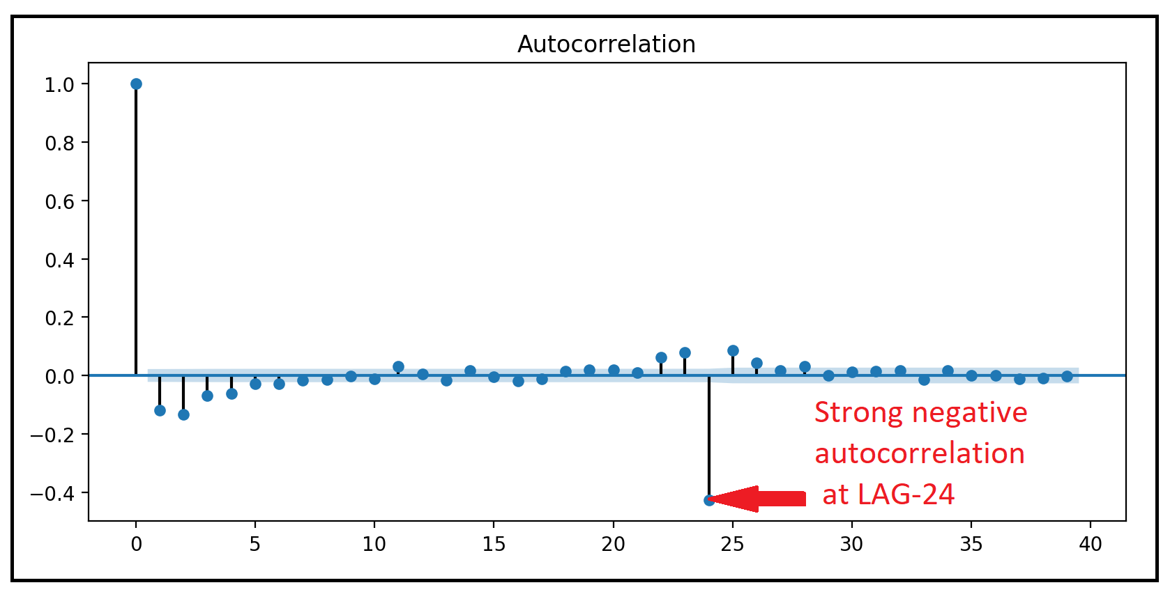

The strong negative correlation at LAG-24 indicates a Seasonal MA (SMA) signature with order 1. i.e. Q=1. Moreover, an absence of positive correlation at LAG-1, indicates an absence of a Seasonal AR component. i.e. P=0.

LAG-24处的强负相关性指示季节性MA(SMA)签名为1阶，即Q = 1 。 此外， 在LAG-1处不存在正相关，表明不存在季节性AR成分。 即P = 0。

We have fixed P=0, D=1 and Q=1, and m=24 hours

我们固定了P = 0，D = 1和Q = 1，并且m = 24小时

That’s it.

而已。

We have managed to estimate all 7 params of the SARIMA model as follows:p=1, d=1, q=0, P=0, D=1, Q=1 and m=24 i.e. SARIMAX(1,1,0)(0,1,1)24

我们设法估计了SARIMA模型的所有7个参数，如下所示： p = 1，d = 1，q = 0，P = 0，D = 1，Q = 1和m = 24，即SARIMAX(1,1,0 )(0,1,1)24

步骤4：建立并拟合具有季节性ARIMA错误的回归模型 (STEP 4: Build and fit the Regression Model with Seasonal ARIMA errors)

Let’s fit the SARIMAX model on the training data set (y_train, X_train) using the above parameters. Before we do that, we need to remove the intercept that Patsy had auto-added to X_train and reset the time series index frequency to Hourly on both X_train and y_train.

让我们使用上述参数将SARIMAX模型拟合到训练数据集( y_train ， X_train )上。 我们这样做之前，我们需要去掉截距懦夫有自动添加到X_train和时间序列索引频率恢复到每小时两个X_train和y_train。

X_train_minus_intercept = X_train.drop('Intercept', axis=1)X_train_minus_intercept = X_train_minus_intercept.asfreq('H')y_train = y_train.asfreq('H')

Let’s build and test the SARIMAX model:

让我们构建和测试SARIMAX模型：

sarimax_model = ARIMA(endog=y_train, exog=X_train_minus_intercept,order=(1,1,0), seasonal_order=(0,1,1,24))sarimax_results = sarimax_model.fit()sarimax_results.summary()

Here’s the training summary:

这是培训摘要：

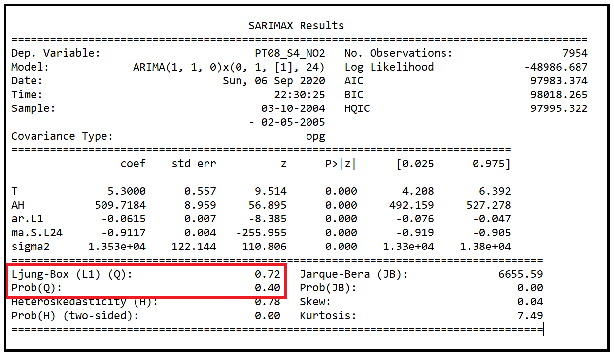
The number to look at first in the training summary is the Ljung-Box test’s statistic and its p-value. The Ljung-Box helps us determine if the residual errors of regression are auto-correlated in a statistically significant way. In this case, the p value is 0.4. So we can rule out auto-correlation in the residual errors at only a 60% confidence level.

训练总结中首先要看的数字是Ljung-Box检验的统计量及其p值。 Ljung-Box可帮助我们确定回归的残差是否以统计学上显着的方式自相关。 在这种情况下，p值为0.4。 因此，我们可以排除仅60％置信水平下残留误差的自相关。

This is rather disappointing and it tells us that we need to experiment with a different combination of parameters for p,d,q,P,D,Q and m. It turns out, this sort of an iteration with different SARIMAX models is not unusual in the SARIMAX world.

这非常令人失望，它告诉我们需要对p，d，q，P，D，Q和m使用不同的参数组合进行实验。 事实证明，在不同的SARIMAX模型中进行这种迭代在SARIMAX世界中并不罕见。

What we’ll do is to simplify our model by setting Q to 0. i.e. we’ll try a SARIMAX(1,1,0)(0,1,0)24 model:

我们要做的是通过将Q设置为0来简化模型。即，我们将尝试SARIMAX(1,1,0)(0,1,0)24模型：

sarimax_model = ARIMA(endog=y_train, exog=X_train_minus_intercept,order=(1,1,0), seasonal_order=(0,1,0,24))sarimax_results = sarimax_model.fit()sarimax_results.summary()

Here’s the training summary:

这是培训摘要：

We see that the p-value of Ljung-Box test statistic has reduced to 0.1 causing us to accept the null hypothesis of the test that the residual errors of regression are not auto-correlated at a 90% confidence level. We can live with this confidence level.

我们看到，Ljung-Box检验统计量的p值已降至0.1，这使我们接受了检验的零假设：回归的残留误差在90％的置信水平下不是自动相关的。 我们可以忍受这个信心水平。

We also see that the residual errors of this second SARIMAX model have other kinds of desirable properties. They are homoscedastic i.e. they have constant variance, as evidenced by the p-value of the homoscedasticity test. Further, the Jarque-Bera test of normality’s test statistic also has a p-value of 0 indicating that the residual errors are normally distributed.

我们还看到，第二个SARIMAX模型的残差具有其他种类的理想属性。 它们是同调的，即它们具有恒定的方差，如同调检验的p值所证明的。 此外，正态性的检验统计量的Jarque-Bera检验也具有p值0，表示残留误差呈正态分布。

In summary, the residual errors of regression of this model are mostly not auto-correlated, they are homoscedastic and normally distributed. The properties of the residuals indicate a high goodness-of-fit.

综上所述，该模型的回归残差大多数不是自相关的，它们是同调的并且是正态分布的。 残差的性质表明拟合优度高。

Finally, note that regression coefficients of all model parameters have a p-value of basically 0 (P > |z| column) indicating a high level of statistical significance.

最后，请注意，所有模型参数的回归系数的p值基本上为0(P> | z |列)，表示具有较高的统计意义。

We’ll accept the SARIMAX(1,1,0)(0,1,0)24 model.

我们将接受SARIMAX(1,1,0)(0,1,0)24模型。

步骤5：预测 (STEP 5: Prediction)

The final step in our SARIMAX saga is using the chosen model to generate some predictions. We’ll ask the model to generate 24 out-of-sample predictions i.e. predict the value of the y (pollutant PT08_S4_NO2) for the next 24 hours beyond the end of the training data set. We’ll use the testing data set (y_test, X_test) which we had carved out in STEP-1. Recollect that the model has never seen the test data set during training.

SARIMAX传奇的最后一步是使用所选模型来生成一些预测。 我们将要求模型生成24个样本外预测，即在训练数据集结束后的接下来的24小时内预测y (污染物PT08_S4_NO2)的值。 我们将使用在STEP-1中确定的测试数据集( y_test ， X_test )。 回忆一下模型在训练期间从未见过测试数据集。

Let’s prepare the test data set for prediction:

让我们准备测试数据集以进行预测：

X_test_minus_intercept = X_test.drop('Intercept', axis=1)X_test_minus_intercept = X_test_minus_intercept.asfreq('H')y_test = y_test.asfreq('H')

Call the get_forecast method to get the out of sample forecasts:

调用get_forecast方法获取样本预测：

predictions = sarimax_results.get_forecast(steps=24, exog=X_test_minus_intercept[:24])predictions.summary_frame()

We get the following output:

我们得到以下输出：

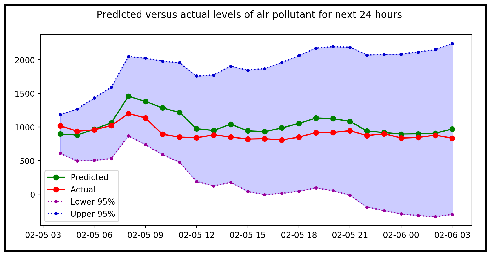
Let’s plot the actual value y_test from the test data set alongside the forecast value mentioned in the ‘mean’ column of the summary _frame. We’ll plot the lower and upper confidence intervals for each forecast value:

让我们将测试数据集的实际值y_test与摘要_frame的“平均值”列中提到的预测值一起绘制。 我们将绘制每个预测值的上下置信区间：

predicted, = plt.plot(X_test_minus_intercept[:24].index, predictions.summary_frame()['mean'], 'go-', label='Predicted')actual, = plt.plot(X_test_minus_intercept[:24].index, y_test[:24], 'ro-', label='Actual')lower, = plt.plot(X_test_minus_intercept[:24].index, predictions.summary_frame()['mean_ci_lower'], color='#990099', marker='.', linestyle=':', label='Lower 95%')upper, = plt.plot(X_test_minus_intercept[:24].index, predictions.summary_frame()['mean_ci_upper'], color='#0000cc', marker='.', linestyle=':', label='Upper 95%')plt.fill_between(X_test_minus_intercept[:24].index, predictions.summary_frame()['mean_ci_lower'], predictions.summary_frame()['mean_ci_upper'], color = 'b', alpha = 0.2)plt.legend(handles=[predicted, actual, lower, upper])plt.show()

We get the following plot:

我们得到以下图：

重要要点 (Key Takeaways)

• Regression with (Seasonal) ARIMA errors (SARIMAX) is a time series regression model that brings together two powerful regression models namely, Linear Regression, and ARIMA (or Seasonal ARIMA).具有(季节性)ARIMA错误的回归(SARIMAX)是一个时间序列回归模型，将两个强大的回归模型(线性回归和ARIMA(或季节性ARIMA))结合在一起。

• The Python Statsmodels library provides powerful support for building (S)ARIMAX models via the statsmodels.tsa.arima.model.ARIMA class in v0.12.0 of statsmodels, or via statsmodels.tsa.statespace.sarimax.SARIMAX in v0.13.0.

  Python Statsmodels库通过statsmodels.tsa.arima.model.ARIMA中的statsmodels.tsa.arima.model.ARIMA类或statsmodels.tsa.statespace.sarimax.SARIMAX中的statsmodels.tsa.statespace.sarimax.SARIMAX为构建(S)ARIMAX模型提供了强大的支持。

• While configuring the (S)ARIMA portion of the (S)ARIMAX model, it helps to use a set of well-known rules (combined with personal judgement) for fixing the values of the p,d,q,P,D,Q and m parameters of the (S)ARIMAX model.在配置(S)ARIMAX模型的(S)ARIMA部分时，它有助于使用一组众所周知的规则(结合个人判断)来固定p，d，q，P，D，Q的值(S)ARIMAX模型的m个参数。
• A well designed (S)ARIMAX model’s residual errors of regression will have very little auto-correlation. This is indicated by the p value of the Ljung-Box test.精心设计的(S)ARIMAX模型的回归残留误差将几乎没有自相关。 这通过Ljung-Box测试的p值表示。
• Additionally, you would want the residual errors to be homoscedastic, and (preferably) normally distributed. So you may have to experiment with different combinations of p,d,q,P,D,Q until you get a model with the best goodness-of-fit characteristics.此外，您可能希望残差是同余的，并且(最好是)正态分布。 因此，您可能必须尝试使用​​p，d，q，P，D，Q的不同组合，直到获得具有最佳拟合优度特征的模型。

相关阅读 (Related reading)

参考，引用和版权 (References, Citations and Copyrights)

Data set of Air Quality measurements is from UCI Machine Learning repository and available for research purposes.

空气质量测量数据集来自UCI机器学习存储库 ，可用于研究目的。

Paper link: S. De Vito, E. Massera, M. Piga, L. Martinotto, G. Di Francia, On field calibration of an electronic nose for benzene estimation in an urban pollution monitoring scenario, Sensors and Actuators B: Chemical, Volume 129, Issue 2, 22 February 2008, Pages 750–757, ISSN 0925–4005, [Web Link]. ([Web Link])

论文链接： S. De Vito，E。Massera，M。Piga，L。Martinotto，G。Di Francia，关于在城市污染监测场景中估算苯的电子鼻的现场校准，传感器和执行器B：化学，体积129，第2期，2008年2月22日，第750-757页，ISSN 0925-4005， [Web链接] 。 ( [Web链接] )

All images in this article are copyright Sachin Date under CC-BY-NC-SA, unless a different source and copyright are mentioned underneath the image.

本文中的所有图像均为CC-BY-NC-SA下的版权Sachin Date ，除非在图像下方提及其他来源和版权。

Thanks for reading! If you liked this article, please follow me to receive tips, how-tos and programming advice on regression and time series analysis.

谢谢阅读！ 如果您喜欢本文，请 关注我 以获取有关回归和时间序列分析的提示，操作方法和编程建议。