史上最详细的XGBoost实战

0. 环境介绍
Python 版本： 3.6.2
操作系统　　： Windows
集成开发环境： PyCharm
1. 安装Python环境
安装Python
首先，我们需要安装Python环境。本人选择的是64位版本的Python 3.6.2。去Python官网https://www.python.org/选择相应的版本并下载。如下如所示：

![这里写图片描述](https://imgconvert.csdnimg.cn/aHR0cDovL2ltZy5ibG9nLmNzZG4ubmV0LzIwMTcxMDAzMTkyNTQ3NTM0?x-oss-process=image/format,png)
接下来安装，并最终选择将Python加入环境变量中。
安装依赖包
去网址：http://www.lfd.uci.edu/~gohlke/pythonlibs/中去下载你所需要的如下Python安装包：
numpy-1.13.1+mkl-cp36-cp36m-win_amd64.whl
scipy-0.19.1-cp36-cp36m-win_amd64.whl
xgboost-0.6-cp36-cp36m-win_amd64.whl
1
2
3
假设上述三个包所在的目录为D:\Application，则运行Windows 命令行运行程序cmd，并将当前目录转到这两个文件所在的目录下。并依次执行如下操作安装这两个包：

>> pip install numpy-1.13.1+mkl-cp36-cp36m-win_amd64.whl
>> pip install scipy-0.19.1-cp36-cp36m-win_amd64.whl
>> pip install xgboost-0.6-cp36-cp36m-win_amd64.whl
1
2
3
安装Scikit-learn

众所周知，scikit-learn是Python机器学习最著名的开源库之一。因此，我们需要安装此库。执行如下命令安装scikit-learn机器学习库：

>> pip install -U scikit-learn
1
测试安装是否成功
>>> from sklearn import svm
>>> X = [[0, 0], [1, 1]]
>>> y = [0, 1]
>>> clf = svm.SVC()
>>> clf.fit(X, y)
>>> clf.predict([[2., 2.]])
array([1])
>>> import xgboost as xgb
1
2
3
4
5
6
7
8
注意：如果如上所述正确输出，则表示安装完成。否则就需要检查安装步骤是否出错，或者系统是否缺少必要的Windows依赖库。常用的一般情况会出现缺少VC++运行库，在Windows 7、8、10等版本中安装Visual C++ 2015基本上就能解决问题。

安装PyCharm

对于PyChram的下载，请点击PyCharm官网去下载，当然windows下软件的安装不用解释，傻瓜式的点击下一步就行了。

![这里写图片描述](https://imgconvert.csdnimg.cn/aHR0cDovL2ltZy5ibG9nLmNzZG4ubmV0LzIwMTcxMDAzMTk1NTI1NTU2?x-oss-process=image/format,png)
注意：PyCharm软件是基于Java开发的，所以安装该集成开发环境前请先安装JDK，建议安装JDK1.8。

经过上述步骤，基本上软件环境的问题全部解决了，接下来就是实际的XGBoost库实战了……

2. XGBoost的优点
2.1 正则化
XGBoost在代价函数里加入了正则项，用于控制模型的复杂度。正则项里包含了树的叶子节点个数、每个叶子节点上输出的score的L2模的平方和。从Bias-variance tradeoff角度来讲，正则项降低了模型的variance，使学习出来的模型更加简单，防止过拟合，这也是xgboost优于传统GBDT的一个特性。

2.2 并行处理
XGBoost工具支持并行。Boosting不是一种串行的结构吗?怎么并行的？注意XGBoost的并行不是tree粒度的并行，XGBoost也是一次迭代完才能进行下一次迭代的（第t次迭代的代价函数里包含了前面t-1次迭代的预测值）。XGBoost的并行是在特征粒度上的。

我们知道，决策树的学习最耗时的一个步骤就是对特征的值进行排序（因为要确定最佳分割点），XGBoost在训练之前，预先对数据进行了排序，然后保存为block结构，后面的迭代中重复地使用这个结构，大大减小计算量。这个block结构也使得并行成为了可能，在进行节点的分裂时，需要计算每个特征的增益，最终选增益最大的那个特征去做分裂，那么各个特征的增益计算就可以开多线程进行。

2.3 灵活性
XGBoost支持用户自定义目标函数和评估函数，只要目标函数二阶可导就行。

2.4 缺失值处理
对于特征的值有缺失的样本，xgboost可以自动学习出它的分裂方向

2.5 剪枝
XGBoost 先从顶到底建立所有可以建立的子树，再从底到顶反向进行剪枝。比起GBM，这样不容易陷入局部最优解。

2.6 内置交叉验证
XGBoost允许在每一轮boosting迭代中使用交叉验证。因此，可以方便地获得最优boosting迭代次数。而GBM使用网格搜索，只能检测有限个值。

3. XGBoost详解
3.1 数据格式
XGBoost可以加载多种数据格式的训练数据：

libsvm 格式的文本数据；

Numpy 的二维数组；

XGBoost 的二进制的缓存文件。加载的数据存储在对象 **DMatrix **中。

下面一一列举：

加载libsvm格式的数据
>>> dtrain1 = xgb.DMatrix('train.svm.txt')
1
加载二进制的缓存文件
>>> dtrain2 = xgb.DMatrix('train.svm.buffer')
1
加载numpy的数组
>>> data = np.random.rand(5,10) # 5 entities, each contains 10 features
>>> label = np.random.randint(2, size=5) # binary target
>>> dtrain = xgb.DMatrix( data, label=label)
1
2
3
将scipy.sparse格式的数据转化为 DMatrix 格式
>>> csr = scipy.sparse.csr_matrix( (dat, (row,col)) )
>>> dtrain = xgb.DMatrix( csr )
1
2
将 DMatrix 格式的数据保存成XGBoost的二进制格式，在下次加载时可以提高加载速度，使用方式如下
>>> dtrain = xgb.DMatrix('train.svm.txt')
>>> dtrain.save_binary("train.buffer")
1
2
可以用如下方式处理 DMatrix中的缺失值：
>>> dtrain = xgb.DMatrix( data, label=label, missing = -999.0)
1
当需要给样本设置权重时，可以用如下方式
>>> w = np.random.rand(5,1)
>>> dtrain = xgb.DMatrix( data, label=label, missing = -999.0, weight=w)
1
2
3.2 参数设置
XGBoost使用key-value字典的方式存储参数：

params = {
'booster': 'gbtree',
'objective': 'multi:softmax', # 多分类的问题
'num_class': 10, # 类别数，与 multisoftmax 并用
'gamma': 0.1, # 用于控制是否后剪枝的参数,越大越保守，一般0.1、0.2这样子。
'max_depth': 12, # 构建树的深度，越大越容易过拟合
'lambda': 2, # 控制模型复杂度的权重值的L2正则化项参数，参数越大，模型越不容易过拟合。
'subsample': 0.7, # 随机采样训练样本
'colsample_bytree': 0.7, # 生成树时进行的列采样
'min_child_weight': 3,
'silent': 1, # 设置成1则没有运行信息输出，最好是设置为0.
'eta': 0.007, # 如同学习率
'seed': 1000,
'nthread': 4, # cpu 线程数
}
1
2
3
4
5
6
7
8
9
10
11
12
13
14
15
3.3 训练模型
有了参数列表和数据就可以训练模型了

num_round = 10
bst = xgb.train( plst, dtrain, num_round, evallist )
1
2
3.4 模型预测
# X_test类型可以是二维List，也可以是numpy的数组
dtest = DMatrix(X_test)
ans = model.predict(dtest)
1
2
3
3.5 保存模型
在训练完成之后可以将模型保存下来，也可以查看模型内部的结构
bst.save_model('test.model')
1
导出模型和特征映射（Map）
你可以导出模型到txt文件并浏览模型的含义：

# dump model
bst.dump_model('dump.raw.txt')
# dump model with feature map
bst.dump_model('dump.raw.txt','featmap.txt')
1
2
3
4
3.6 加载模型
通过如下方式可以加载模型：

bst = xgb.Booster({'nthread':4}) # init model
bst.load_model("model.bin") # load data
1
2
4. XGBoost参数详解
在运行XGboost之前，必须设置三种类型成熟：general parameters，booster parameters和task parameters：

General parameters
该参数参数控制在提升（boosting）过程中使用哪种booster，常用的booster有树模型（tree）和线性模型（linear model）。

Booster parameters
这取决于使用哪种booster。

Task parameters
控制学习的场景，例如在回归问题中会使用不同的参数控制排序。

4.1 General Parameters
booster [default=gbtree]
有两中模型可以选择gbtree和gblinear。gbtree使用基于树的模型进行提升计算，gblinear使用线性模型进行提升计算。缺省值为gbtree

silent [default=0]
取0时表示打印出运行时信息，取1时表示以缄默方式运行，不打印运行时信息。缺省值为0

**nthread **
XGBoost运行时的线程数。缺省值是当前系统可以获得的最大线程数

num_pbuffer
预测缓冲区大小，通常设置为训练实例的数目。缓冲用于保存最后一步提升的预测结果，无需人为设置。

**num_feature **
Boosting过程中用到的特征维数，设置为特征个数。XGBoost会自动设置，无需人为设置。

4.2 Parameters for Tree Booster
eta [default=0.3]
为了防止过拟合，更新过程中用到的收缩步长。在每次提升计算之后，算法会直接获得新特征的权重。 eta通过缩减特征的权重使提升计算过程更加保守。缺省值为0.3
取值范围为：[0,1]

gamma [default=0]
minimum loss reduction required to make a further partition on a leaf node of the tree. the larger, the more conservative the algorithm will be.
取值范围为：[0,∞]

max_depth [default=6]
数的最大深度。缺省值为6
取值范围为：[1,∞]

min_child_weight [default=1]
孩子节点中最小的样本权重和。如果一个叶子节点的样本权重和小于min_child_weight则拆分过程结束。在现行回归模型中，这个参数是指建立每个模型所需要的最小样本数。该成熟越大算法越conservative
取值范围为：[0,∞]

max_delta_step [default=0]
我们允许每个树的权重被估计的值。如果它的值被设置为0，意味着没有约束；如果它被设置为一个正值，它能够使得更新的步骤更加保守。通常这个参数是没有必要的，但是如果在逻辑回归中类极其不平衡这时候他有可能会起到帮助作用。把它范围设置为1-10之间也许能控制更新。
取值范围为：[0,∞]

subsample [default=1]
用于训练模型的子样本占整个样本集合的比例。如果设置为0.5则意味着XGBoost将随机的从整个样本集合中随机的抽取出50%的子样本建立树模型，这能够防止过拟合。
取值范围为：(0,1]

colsample_bytree [default=1]
在建立树时对特征采样的比例。缺省值为1
取值范围为：(0,1]

4.3 Parameter for Linear Booster
lambda [default=0]
L2 正则的惩罚系数

alpha [default=0]
L1 正则的惩罚系数

lambda_bias
在偏置上的L2正则。缺省值为0（在L1上没有偏置项的正则，因为L1时偏置不重要）

4.4 Task Parameters
objective [ default=reg:linear ]
定义学习任务及相应的学习目标，可选的目标函数如下：

“reg:linear” —— 线性回归。

“reg:logistic”—— 逻辑回归。

“binary:logistic”—— 二分类的逻辑回归问题，输出为概率。

“binary:logitraw”—— 二分类的逻辑回归问题，输出的结果为wTx。

“count:poisson”—— 计数问题的poisson回归，输出结果为poisson分布。在poisson回归中，max_delta_step的缺省值为0.7。(used to safeguard optimization)

“multi:softmax” –让XGBoost采用softmax目标函数处理多分类问题，同时需要设置参数num_class（类别个数）

“multi:softprob” –和softmax一样，但是输出的是ndata * nclass的向量，可以将该向量reshape成ndata行nclass列的矩阵。没行数据表示样本所属于每个类别的概率。

“rank:pairwise” –set XGBoost to do ranking task by minimizing the pairwise loss

base_score [ default=0.5 ]

所有实例的初始化预测分数，全局偏置；
为了足够的迭代次数，改变这个值将不会有太大的影响。
eval_metric [ default according to objective ]

校验数据所需要的评价指标，不同的目标函数将会有缺省的评价指标（rmse for regression, and error for classification, mean average precision for ranking）-

用户可以添加多种评价指标，对于Python用户要以list传递参数对给程序，而不是map参数list参数不会覆盖’eval_metric’

可供的选择如下:

“rmse”: root mean square error
“logloss”: negative log-likelihood
“error”: Binary classification error rate. It is calculated as #(wrong cases)/#(all cases). For the predictions, the evaluation will regard the instances with prediction value larger than 0.5 as positive instances, and the others as negative instances.
“merror”: Multiclass classification error rate. It is calculated as #(wrongcases)#(allcases)\frac{\#(wrong \quad cases)}{\#(all \quad cases)}
#(allcases)
#(wrongcases)

.
“mlogloss”: Multiclass logloss
“auc”: Area under the curve for ranking evaluation.
“ndcg”:Normalized Discounted Cumulative Gain
“map”:Mean average precision
“ndcg@n”,”map@n”: n can be assigned as an integer to cut off the top positions in the lists for evaluation.
“ndcg-“,”map-“,”ndcg@n-“,”map@n-“: In XGBoost, NDCG and MAP will evaluate the score of a list without any positive samples as 1. By adding “-” in the evaluation metric XGBoost will evaluate these score as 0 to be consistent under some conditions. training repeatively
seed [ default=0 ]

随机数的种子。缺省值为0
5. XGBoost实战
XGBoost有两大类接口：XGBoost原生接口和 scikit-learn接口，并且XGBoost能够实现分类和回归两种任务。因此，本章节分四个小块来介绍！

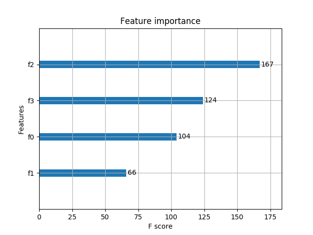
5.1 基于XGBoost原生接口的分类
from sklearn.datasets import load_iris
import xgboost as xgb
from xgboost import plot_importance
from matplotlib import pyplot as plt
from sklearn.model_selection import train_test_split

# read in the iris data
iris = load_iris()

X = iris.data
y = iris.target

X_train, X_test, y_train, y_test = train_test_split(X, y, test_size=0.2, random_state=1234565)

params = {
'booster': 'gbtree',
'objective': 'multi:softmax',
'num_class': 3,
'gamma': 0.1,
'max_depth': 6,
'lambda': 2,
'subsample': 0.7,
'colsample_bytree': 0.7,
'min_child_weight': 3,
'silent': 1,
'eta': 0.1,
'seed': 1000,
'nthread': 4,
}

plst = params.items()

dtrain = xgb.DMatrix(X_train, y_train)
num_rounds = 500
model = xgb.train(plst, dtrain, num_rounds)

# 对测试集进行预测
dtest = xgb.DMatrix(X_test)
ans = model.predict(dtest)

# 计算准确率
cnt1 = 0
cnt2 = 0
for i in range(len(y_test)):
if ans[i] == y_test[i]:
cnt1 += 1
else:
cnt2 += 1

print("Accuracy: %.2f %% " % (100 * cnt1 / (cnt1 + cnt2)))

# 显示重要特征
plot_importance(model)
plt.show()

1
2
3
4
5
6
7
8
9
10
11
12
13
14
15
16
17
18
19
20
21
22
23
24
25
26
27
28
29
30
31
32
33
34
35
36
37
38
39
40
41
42
43
44
45
46
47
48
49
50
51
52
53
54
55
56
输出预测正确率以及特征重要性：

Accuracy: 96.67 %
1
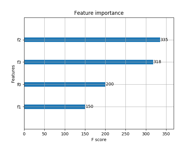
![这里写图片描述](https://imgconvert.csdnimg.cn/aHR0cDovL2ltZy5ibG9nLmNzZG4ubmV0LzIwMTcxMDIyMTQyNDQyODIw?x-oss-process=image/format,png)
5.2 基于XGBoost原生接口的回归
import xgboost as xgb
from xgboost import plot_importance
from matplotlib import pyplot as plt
from sklearn.model_selection import train_test_split

# 读取文件原始数据
data = []
labels = []
labels2 = []
with open("lppz5.csv", encoding='UTF-8') as fileObject:
for line in fileObject:
line_split = line.split(',')
data.append(line_split[10:])
labels.append(line_split[8])

X = []
for row in data:
row = [float(x) for x in row]
X.append(row)

y = [float(x) for x in labels]

# XGBoost训练过程
X_train, X_test, y_train, y_test = train_test_split(X, y, test_size=0.2, random_state=0)

params = {
'booster': 'gbtree',
'objective': 'reg:gamma',
'gamma': 0.1,
'max_depth': 5,
'lambda': 3,
'subsample': 0.7,
'colsample_bytree': 0.7,
'min_child_weight': 3,
'silent': 1,
'eta': 0.1,
'seed': 1000,
'nthread': 4,
}

dtrain = xgb.DMatrix(X_train, y_train)
num_rounds = 300
plst = params.items()
model = xgb.train(plst, dtrain, num_rounds)

# 对测试集进行预测
dtest = xgb.DMatrix(X_test)
ans = model.predict(dtest)

# 显示重要特征
plot_importance(model)
plt.show()
1
2
3
4
5
6
7
8
9
10
11
12
13
14
15
16
17
18
19
20
21
22
23
24
25
26
27
28
29
30
31
32
33
34
35
36
37
38
39
40
41
42
43
44
45
46
47
48
49
50
51
52
重要特征(值越大，说明该特征越重要)显示结果：

![这里写图片描述](https://imgconvert.csdnimg.cn/aHR0cDovL2ltZy5ibG9nLmNzZG4ubmV0LzIwMTcxMDIyMTM1MjQyMTM4?x-oss-process=image/format,png)
5.3 基于Scikit-learn接口的分类
from sklearn.datasets import load_iris
import xgboost as xgb
from xgboost import plot_importance
from matplotlib import pyplot as plt
from sklearn.model_selection import train_test_split

# read in the iris data
iris = load_iris()

X = iris.data
y = iris.target

X_train, X_test, y_train, y_test = train_test_split(X, y, test_size=0.2, random_state=0)

# 训练模型
model = xgb.XGBClassifier(max_depth=5, learning_rate=0.1, n_estimators=160, silent=True, objective='multi:softmax')
model.fit(X_train, y_train)

# 对测试集进行预测
ans = model.predict(X_test)

# 计算准确率
cnt1 = 0
cnt2 = 0
for i in range(len(y_test)):
if ans[i] == y_test[i]:
cnt1 += 1
else:
cnt2 += 1

print("Accuracy: %.2f %% " % (100 * cnt1 / (cnt1 + cnt2)))

# 显示重要特征
plot_importance(model)
plt.show()
1
2
3
4
5
6
7
8
9
10
11
12
13
14
15
16
17
18
19
20
21
22
23
24
25
26
27
28
29
30
31
32
33
34
35
输出预测正确率以及特征重要性：

Accuracy: 100.00 %
1
![这里写图片描述](https://imgconvert.csdnimg.cn/aHR0cDovL2ltZy5ibG9nLmNzZG4ubmV0LzIwMTcxMDIyMTQzMDM1NjIy?x-oss-process=image/format,png)
5.4 基于Scikit-learn接口的回归
import xgboost as xgb
from xgboost import plot_importance
from matplotlib import pyplot as plt
from sklearn.model_selection import train_test_split

X = []
for row in data:
row = [float(x) for x in row]
X.append(row)

y = [float(x) for x in labels]

# XGBoost训练过程
X_train, X_test, y_train, y_test = train_test_split(X, y, test_size=0.2, random_state=0)

model = xgb.XGBRegressor(max_depth=5, learning_rate=0.1, n_estimators=160, silent=True, objective='reg:gamma')
model.fit(X_train, y_train)

# 对测试集进行预测
ans = model.predict(X_test)

# 显示重要特征
plot_importance(model)
plt.show()
1
2
3
4
5
6
7
8
9
10
11
12
13
14
15
16
17
18
19
20
21
22
23
24
25
26
27
28
29
30
31
32
33
34
重要特征(值越大，说明该特征越重要)显示结果：

![这里写图片描述](https://imgconvert.csdnimg.cn/aHR0cDovL2ltZy5ibG9nLmNzZG4ubmV0LzIwMTcxMDIyMTM1ODAyMTg4?x-oss-process=image/format,png)
未完待续……

对机器学习和人工智能感兴趣，请微信扫码关注公众号！
![这里写图片描述](https://imgconvert.csdnimg.cn/aHR0cDovL2ltZy5ibG9nLmNzZG4ubmV0LzIwMTcxMDIxMjM0MzM4MzQx?x-oss-process=image/format,png)
————————————————
版权声明：本文为CSDN博主「JeemyJohn」的原创文章，遵循 CC 4.0 BY-SA 版权协议，转载请附上原文出处链接及本声明。
原文链接：https://blog.csdn.net/u013709270/article/details/78156207

史上最详细的XGBoost实战相关推荐

python xgboost实战_史上最详细的XGBoost实战
0. 环境介绍 Python 版本: 3.6.2 操作系统 : Windows 集成开发环境: PyCharm 1. 安装Python环境安装Python 首先,我们需要安装Python环境.本人 ...
android项目实战博学谷源码_Vue框架：史上最详细的Vue实战项目之喵喵电影（视频+源码）...
Vue是web前端中重要的框架之一,与其他重量级框架不同的是,Vue 采用自底向上增量开发的设计,Vue 的核心库只关注视图层,并且非常容易学习,非常容易与其它库或已有项目整合.所以,对于web前端开 ...
史上最详细阿里云服务器上Docker部署War包项目实战每一步都带详细图解！！！
史上最详细阿里云服务器上Docker部署War包项目实战每一步都带详细图解!!! 部署jar 包方式: https://blog.csdn.net/weixin_45821811/article/d ...
GitChat·大数据 | 史上最详细的Hadoop环境搭建
GitChat 作者:鸣宇淳原文: 史上最详细的Hadoop环境搭建关注公众号:GitChat 技术杂谈,一本正经的讲技术 [不要错过文末彩蛋] 前言 Hadoop在大数据技术体系中的地位至关重要 ...
RISC-V AI芯片Celerity史上最详细解读（上）（附开源地址）
RISC-V AI芯片Celerity史上最详细解读(上)(附开源地址) (本文包括Celerity中二值化神经网络的介绍) 作者陈巍,资深芯片专家,人工智能算法-硬件协同设计专家. 在Hot Ch ...
史上最详细的微生物扩增子数据库整理
声明:文件所有链接内容来自"生信控"公众号,已经获作者向屿授权. 本人对每个数据库的使用目的和经验配导读,需要使用的小伙伴读点击链接跳转原文学习. "生信控"相 ...
史上最详细版Centos6安装详细教程
镜像CentOS-6.8-x86_64-bin-DVD1.ISO 将下载好的镜像上传到服务器,并选择该镜像(详情请看上篇exsi镜像上传文章) 一.安装开始开机选择第一项这里询问我们是否要对光盘进 ...
史上最详细“截图”搭建Hexo博客——For Windows
http://angelen.me/2015/01/23/2015-01-23-%E5%8F%B2%E4%B8%8A%E6%9C%80%E8%AF%A6%E7%BB%86%E2%80%9C%E6%88 ...
不仅有史上最详细Docker 安装Minio Client，还附带解决如何设置永久访问和永久下载链接！！（详图）绝对值得收藏的哈！！！！
背景: 这两天在整理知识点,然后在学习Minio,一开始遇到更新,整了我不少时间,之前用的太久了,改了不少东西.用了之后发现不知道怎么设置成永久访问,就出了这篇文章. 史上最详细Docker安装最新版 ...

史上最详细的XGBoost实战

史上最详细的XGBoost实战相关推荐

最新文章

热门文章