Update: This post is part of a blog series on Meta-Learning that I’m working on. Check out part 1 and part 2.

更新 ：这篇文章是我正在从事的有关元学习的博客系列的一部分。 检出 第1 部分 和 第2部分 。

In my previous post, “Meta-Learning Is All You Need,” I discussed the motivation for the meta-learning paradigm, explained the mathematical underpinning, and reviewed the three approaches to design a meta-learning algorithm (namely, black-box, optimization-based, and non-parametric).

在我之前的文章“ 元学习就是您所需要的 ”中，我讨论了元学习范式的动机，解释了数学基础，并回顾了设计元学习算法的三种方法(即黑盒 ， 基于优化的和非参数的 )。

I also mentioned in the post that there are two views of the meta-learning problem: a deterministic view and a probabilistic view, according to Chelsea Finn.

在切尔西·芬 ( Chelsea Finn)的文章中，我还提到过元学习问题有两种观点：确定性观点和概率观点。

• The deterministic view is straightforward: we take as input a training data set Dᵗʳ, a test data point, and the meta-parameters θ to produce the label corresponding to that test input.

  确定性视图很简单：我们将训练数据集Dᵗʳ，测试数据点和元参数θ作为输入，以产生与该测试输入相对应的标签。

• The probabilistic view incorporates Bayesian inference: we perform a maximum likelihood inference over the task-specific parameters ϕᵢ — assuming that we have the training dataset Dᵢᵗʳ and a set of meta-parameters θ.

  概率视图包含贝叶斯推断：我们对特定于任务的参数进行最大似然推断-假设我们有训练数据集Dᵢᵗʳ和一组元参数θ。

This blog post is my attempt to demystify the probabilistic view and answer these key questions:

这篇博客文章是我试图揭开概率论的神秘面纱，并回答以下关键问题：

1. Why is the deterministic view of meta-learning not sufficient?
   为什么对元学习的确定性看法不足？
2. What is the variational inference?
   什么是变分推理？
3. How can we design neural-based Bayesian meta-learning algorithms?
   我们如何设计基于神经的贝叶斯元学习算法？

Note: The content of this post is primarily based on CS330’s lecture 5 on Bayesian meta-learning. It is accessible to the public.

注意： 这篇文章的内容主要基于CS330 关于贝叶斯元学习 的 讲座5 。 它对公众开放。

1 —确定性元学习的弊端 (1 — The Downsides Of Deterministic Meta-Learning)

Deterministic meta-learning approaches provide us with p(ϕᵢ|Dᵢᵗʳ, θ) — a point estimate of the task-specific parameters ϕᵢ given the training set and the meta-parameters θ. In many situations, we need more than just a point estimate. For example, there are various meta-learning problems that are not entirely determined by their data distribution, as their underlying functions are ambiguous given some prior information. These problems happen in safety-critical domains such as autonomous vehicles and medical imaging, in exploration strategies for meta reinforcement learning, and in active-learning.

确定性元学习方法为我们提供p(ϕᵢ |Dᵢᵗʳ，θ) -给定训练集和元参数θ的任务特定参数point的点估计。 在许多情况下，我们不仅需要点估计。 例如，存在各种元学习问题，这些问题并非完全由其数据分布确定，因为在给定一些先验信息的情况下，其基本功能尚不明确。 这些问题发生在安全关键领域，例如自动驾驶汽车和医学成像，元强化学习的探索策略以及主动学习中。

In particular, active-learning with meta-learning is potentially a research direction with many industry use cases. Active-learning is valuable in cases where the initial amount of labeled data is small — which frequently happens in the messy real-world. This learning paradigm leverages an existing classifier to decide which unlabeled data points that need to be labeled to improve the existing classifier the most. Previous active-learning methods rely heavily on heuristics such as choosing the data points whose label the model is most uncertain about, choosing the data points whose addition will cause the model to be least uncertain about other data points, or choosing the data points that are different compared to others according to a similarity function.

特别地， 具有元学习的主动学习可能是许多行业用例的研究方向。 主动学习在标记数据的初始数量很少的情况下很有价值，而这种情况经常在混乱的现实世界中发生。 该学习范例利用现有分类器来决定哪些标签未标记的数据点需要标记以最大程度地改善现有分类器。 以前的主动学习方法严重依赖启发式方法，例如选择模型不确定性最高的数据点，选择其添加将导致模型对其他数据不确定性最小的数据点，或选择根据相似度函数与其他人相比有所不同。

• Woodward and Finn combine meta-learning with reinforcement learning to learn an active learner. More specifically, the authors considered the online setting of active learning, where the agent is presented with examples in a sequence and must choose whether to label the example or request the correct label. Given the reinforcement learning paradigm, the model is a policy with two actions (labeling and requesting labels) and thus can effectively make decisions with few labeled examples.

  Woodward和Finn将元学习与强化学习相结合，以学习活跃的学习者。 更具体地说，作者考虑了主动学习的在线设置，在该设置中，代理将按顺序显示示例，并且必须选择是标记示例还是请求正确的标签。 在给定强化学习范例的情况下，该模型是具有两个动作(标记和请求标记)的策略，因此可以通过很少的标记示例有效地做出决策。

• Konyushkova et al. introduce a data-driven approach to meta-learning termed Learning Active Learning. Given a trained classifier and its output for a specific example without a label, the authors trained a regressor to predict the reduction in generalization error that can be expected by adding the label to that point. The resulting active learning strategy was then personalized to the specific problem at hand and could be used to further extend to the initial dataset. This query selection strategy outperformed competing methods without requiring hand-crafted heuristics and at a comparatively low computational cost.

  Konyushkova等。 介绍一种称为“ 学习主动学习”的数据驱动的元学习方法。 给定训练有素的分类器及其在没有标签的特定示例中的输出，作者对回归器进行了培训，以预测通过将标签添加到该点可以预期的泛化误差的减少。 然后将得到的主动学习策略个性化以解决当前的特定问题，并可用于进一步扩展到初始数据集。 该查询选择策略在不要求手工制作启发式算法的情况下，以较低的计算成本胜过竞争方法。

• Bachman et al. propose a model that learns active learning algorithms via meta-learning (figure 1). The model interacts with labeled items for many related tasks to discover an active learning strategy for the task at hand. This learned active learning strategy could outperform task-agnostic heuristics by sharing experience across associated tasks. In particular, the authors figured out a way to balance the data representation, the active learning strategy, and the prediction function constructor.

  Bachman等。 提出了一个通过元学习来学习主动学习算法的模型(图1)。 该模型与带有标签的项目交互以执行许多相关任务，以发现针对当前任务的主动学习策略。 通过跨相关任务共享经验，这种学习的主动学习策略可以胜过与任务无关的启发式方法。 特别是，作者找到了一种平衡数据表示，主动学习策略和预测函数构造函数的方法。

We can address the drawbacks of deterministic meta-learning by generating hypotheses about the underlying function, sampling from that data distribution, and reasoning about the model uncertainty. This is where Bayesian meta-learning comes in.

我们可以通过生成有关基础函数的假设，从该数据分布中采样以及对模型不确定性进行推理来解决确定性元学习的弊端。 这就是贝叶斯元学习的地方。

2 —贝叶斯非深度学习元学习者 (2 — A Light Touch On Bayesian Non-Deep Learning Meta-Learners)

Before discussing the meta-learners that utilize deep learning, let us pay respect to the efforts that tackled meta-learning before the neural networks revolution:

在讨论利用深度学习的元学习者之前，让我们尊重神经网络革命之前解决元学习的努力：

• “One-shot Learning of Object Categories” by Fei-Fei, Fergus, and Perona (2006) is one of the earliest approaches that use meta-learning for object recognition tasks. Rather than learning from scratch, the authors took advantage of knowledge coming from previously learned categories, no matter how different these categories might be. This hypothesis was conducted via a Bayesian setting: The authors extracted “general knowledge” from previously learned categories and represented it in the form of a prior probability density function in the space of model parameters. Given a training set, no matter how small, the authors updated this knowledge and produced a posterior density that could be used for object recognition. Their experiments showed that this had been a productive approach and that some useful information about categories could have been obtained from a few training examples.

  Fei-Fei，Fergus和Perona(2006)撰写的“ 对象类别的一次性学习 ”是将元学习用于对象识别任务的最早方法之一。 作者可以从先前学习的类别中获得知识，而不必从头开始学习，无论这些类别可能有多么不同。 该假设是通过贝叶斯环境进行的：作者从先前学习的类别中提取了“一般知识”，并以模型参数空间中的先验概率密度函数的形式表示了该知识。 给定一个训练集，无论大小如何，作者都更新了此知识，并产生了可用于对象识别的后验密度。 他们的实验表明，这是一种有效的方法，并且可以从一些培训示例中获得一些有关类别的有用信息。

• “One-shot Learning of Simple Visual Concepts” by Lake, Salakhutdinov, Gross, and Tenenbaum (2011) works in the domain of handwritten characters, an ideal setting for studying one-shot learning at the interface of human and machine learning. Handwritten characters contain a rich internal part structure of pen strokes, providing good a priori reason to explore a parts-based approach to representation learning. The authors proposed a new model of character learning based on inducing probabilistic part-based representations. Given an example image of a new character type, the model infers a sequence of latent strokes that best explains the pixels in the image, drawing on a broad stroke vocabulary abstracted from many previous characters. This stroke-based representation guides generalization to new examples of the concept.

  Lake，Salakhutdinov，Gross和Tenenbaum(2011)撰写的“ 简单视觉概念的一次性学习 ”在手写字符领域工作，这是在人机学习和机器学习的界面上研究一次性学习的理想环境。 手写字符包含丰富的笔触内部部分结构，这为探索基于部分的表示学习方法提供了很好的先验理由。 作者提出了一种新的基于角色概率表示的字符学习模型。 给定一个新字符类型的示例图像，该模型会根据从许多先前字符中提取的广泛笔触词汇表，推断出一系列潜在笔画，从而最好地解释了图像中的像素。 这种基于笔画的表示法将概括性地引入了该概念的新示例。

• “One-shot Learning with a Hierarchical Nonparametric Bayesian Model” by Salakhutdinov, Tenenbaum, and Torralba (2012) leverages higher-order knowledge abstracted from previously learned categories to estimate the new category’s prototype as well as an appropriate similarity metric from just one example. These estimates are also improved as more examples are observed. As illustrated in figure 2, consider how human learners seeing one example of an unfamiliar animal, such as a “wildebeest,” can draw on experience with many examples of “horse,” “cows,” “sheep,” etc. These similar categories have similar prototypes and share similarity variation in their feature-space representations. If we can identify the new example of “wildebeest” as belonging to this “animal” super-category, we can transfer an appropriate similarity metric and thereby generate informatively even from a single example. The algorithm that the authors used is a general-purpose hierarchical Bayesian model that depends minimally on domain-specific representations but instead learns to perform one-shot learning by finding more intelligent representations tuned to specific sub-domains of a task.

  Salakhutdinov，Tenenbaum和Torralba(2012)撰写的“ 使用分层非参数贝叶斯模型进行一次学习 ”，利用从先前学习的类别中提取的高级知识来估计新类别的原型以及仅通过一个示例得出的适当相似性指标。 随着更多实例的观察，这些估计值也得到了改善。 如图2所示，请考虑人类学习者如何看到一个不熟悉的动物示例，例如“野兽”，可以借鉴许多“马”，“牛”，“绵羊”等示例的经验。这些相似的类别具有相似的原型，并在其特征空间表示中共享相似性变化。 如果我们可以将“野生动物”的新示例识别为属于该“动物”超类别，则可以传递适当的相似性度量，从而即使从单个示例中也能提供有益的信息。 作者使用的算法是通用的分层贝叶斯模型 ，该模型最少依赖于特定于域的表示形式，而是通过查找调整到任务特定子域的更智能的表示来学习执行一次学习。

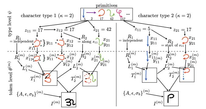
• “One-shot Learning by Inverting A Compositional Causal Process” by Lake, Salakhutdinov, and Tenenbaum (2013) tackles one-shot learning via a computational approach called Hierarchical Bayesian Program Learning that utilizes the principles of compositionally and causality to build a probabilistic generative model of handwritten characters (figure 3). It is compositional because characters are represented as stochastic motor programs where the primitive structure is shared and reused across characters at multiple levels, including strokes and sub-strokes. Given the raw pixels, the model searches for a “structural description” to explain the image by freely combining these elementary parts and their spatial relations. It is causal because strokes are not modeled at the level of muscle movements, but they are abstract enough to be completed by higher-order actions.

  Lake，Salakhutdinov和Tenenbaum(2013)撰写的“ 通过反转组成因果过程进行的一键式学习”通过一种称为“ 层次贝叶斯程序学习”的计算方法来解决一键式学习，该方法利用组成和因果关系的原理来构建概率生成模型手写字符(图3)。 这是组成性的，因为字符被表示为随机运动程序，其中原始结构在多个级别(包括笔划和子笔划)之间跨字符共享和重用。 给定原始像素，模型将通过自由组合这些基本部分及其空间关系来搜索“结构描述”以解释图像。 这是有原因的，因为中风不是在肌肉运动的水平上建模的，但是它们足够抽象，可以通过高阶动作来完成。

3 —贝叶斯深度学习入门 (3 — A Primer On Bayesian Deep Learning)

Deep learning requires a large amount of high-quality data and thus can overfit when the dataset size is small. Other common issues include catastrophic forgetting (the forgetting of past knowledge) and unreliable confidence estimates (lack of robustness and vulnerability to adversarial attacks). Ultimately, due to such issues, real-world applications of deep learning are still challenging.

深度学习需要大量高质量的数据，因此当数据集大小较小时，深度学习可能会过度拟合。 其他常见问题包括灾难性的遗忘(遗忘过去的知识)和不可靠的置信度估计(缺乏鲁棒性和对抗性攻击的脆弱性)。 最终，由于这些问题，深度学习在现实世界中的应用仍然具有挑战性。

Bayesian principles have the potential to address such issues:

贝叶斯原理有可能解决以下问题：

• We can use posterior distribution to represent model uncertainty.
  我们可以使用后验分布来表示模型的不确定性。
• We can use Bayes’ rule to enable sequential learning.
  我们可以使用贝叶斯规则来启用顺序学习。
• We can use Bayesian model averaging to reduce over-fitting.
  我们可以使用贝叶斯模型平均来减少过度拟合。

Despite these benefits, they are rarely employed in practice due to computational concerns of the posterior distribution, which overshadows their theoretical advantages.

尽管有这些好处，但由于后验分布的计算问题，它们在实践中很少使用，这掩盖了它们的理论优势。

So, what are the different approaches to build neural networks that can measure uncertainty?

那么，构建可测量不确定性的神经网络有哪些不同的方法呢？

• A prevalent method is to use latent variable models and optimize them via variational inference. To perform efficient inference and learning in directed probabilistic models, Kingma and Welling introduce a stochastic variational inference and learning algorithm that scales to large datasets and even works in the intractable case. More specifically, the paper comes up with the reparameterization trick to yield a lower bound estimator, which can be used for efficient approximate posterior inference in almost any model with continuous latent variables. Rezende et al. combine ideas from neural networks and probabilistic latent variable modeling to derive a general class of Deep Latent Gaussian models (shown in figure 4), which are principally directed graphical models that consist of Gaussian latent variables at each layer of a processing hierarchy. Furthermore, the paper presents an approach for a scalable variational inference that allows for joint optimization of both variational and model parameters by exploring the properties of latent Gaussian distributions and gradient back-propagation.

  一种普遍的方法是使用潜在变量模型，并通过变分推断对其进行优化 。 为了在定向概率模型中执行有效的推理和学习， Kingma和Welling引入了一种随机变分推理和学习算法，该算法可以扩展到大型数据集，甚至可以在难处理的情况下工作。 更具体地说，本文提出了重新参数化技巧，以产生下界估计量，该估计量可用于几乎任何具有连续潜在变量的模型中的有效近似后验推断。 Rezende等。 结合神经网络和概率潜在变量建模的思想，可以得出一类通用的深度潜在高斯模型 (如图4所示)，这些模型主要是有向图模型，由在处理层次结构每一层上的高斯潜在变量组成。 此外，本文提出了一种可扩展的变分推论方法，该方法可以通过探索潜在的高斯分布和梯度反向传播的属性来联合优化变分和模型参数。

• Another method is to use an ensemble to estimate the model uncertainty. Lakshminarayanan et al. describe a simple and scalable non-Bayesian method for determining predictive uncertainty estimates from neural networks. The technique uses a combination of ensembles (which captures “model uncertainty” by averaging predictions over multiple models consistent with the training data), and adversarial training (which encourages local smoothness), for robustness to model misspecification and out-of-distribution examples. This method requires minimal hyper-parameter tuning and is well suited for large-scale distributed computation and can be readily implemented for a wide variety of architectures.

  另一种方法是使用整体估计模型不确定性。 Lakshminarayanan等。 描述了一种简单且可扩展的非贝叶斯方法，用于从神经网络确定预测不确定性估计。 该技术结合使用了合奏 (通过对与训练数据一致的多个模型的预测结果取平均值来捕获“模型不确定性”)和对抗性训练 (鼓励局部平滑度)，以增强模型失误和分布失调示例的鲁棒性。 该方法需要最少的超参数调整，非常适合于大规模分布式计算，并且可以很容易地实现各种体系结构。

• The next method is to represent an explicit distribution over the weights of the neural network parameters. Blundell et al. introduce an algorithm called Bayes by Backbrop that learns the weights of neural networks with uncertainty. It optimizes a well-defined objective function to learn a distribution on the weights (shown in figure 5). The paper argues that introducing uncertainty on the weights: (1) helps with regularization via a compression cost on the weights, (2) provides richer representations and predictions from cheap model averaging, and (3) assists with exploration strategies in simple reinforcement learning problems such as contextual bandits.

  下一种方法是表示神经网络参数权重上的显式分布。 Blundell等。 引入了Backbrop称为Bayes的算法，该算法学习具有不确定性的神经网络的权重。 它优化了定义明确的目标函数，以学习权重的分布(如图5所示)。 本文认为在权重上引入不确定性：(1)通过权重上的压缩成本帮助进行正则化；(2)通过廉价的模型平均提供更丰富的表示和预测；(3)在简单的强化学习问题中协助探索策略例如情境强盗。

• We can also use normalizing flows: a class of models that attempt to represent a function over a data distribution by (1) inverting some latent distribution into the data distribution or (2) transforming from latent space into the data space and back into the latent space. Dinh et al. propose Non-Linear Independent Component Estimation (NICE), a normalizing flow model type that can model complex high-dimensional densities. Its architecture is capable of learning a highly non-linear bijective transformation (that maps the training data to space where its distribution is factorized) via maximum log-likelihood. The authors also noted that NICE could enable robust approximate inference allowing a complex family of approximate posterior distributions in variational auto-encoders.

  我们还可以使用归一化流：试图通过以下方式表示数据分布上的函数的一类模型：(1)将某些潜在分布转换为数据分布，或者(2)从潜在空间转换为数据空间然后再转换为潜在空间空间。 Dinh等。 提出了非线性独立分量估计(NICE)，这是一种可以对复杂的高维密度建模的标准化流模型类型。 它的体系结构能够通过最大对数似然来学习高度非线性的双射变换(将训练数据映射到其分布被分解的空间)。 作者还指出，NICE可以实现鲁棒的近似推理，从而在变分自动编码器中允许复杂的近似后验分布族。

• Finally, we have energy-based models. Energy-Based models capture dependencies between variables by associating scalar energy to each configuration of the variables. At inference time, we set the value of those observed variables and find the values of the remaining variables that minimize the energy. At training time, we find an energy function that associates low energies to correct values of the remaining variables and higher energies to incorrect values. Because there is no requirement for proper normalization, energy-based approaches avoid the problem associated with estimating the normalization constant in probabilistic models. Furthermore, the absence of the normalization condition allows for much more flexibility in the design of learning machines. Generative adversarial networks are a popular type of energy-based models.

  最后，我们有基于能量的模型 。 基于能量的模型通过将标量能量与变量的每个配置相关联来捕获变量之间的依赖性。 在推断时，我们设置那些观测变量的值，并找到使能量最小化的其余变量的值。 在训练时，我们发现一个能量函数，该函数将低能量关联到剩余变量的正确值，而将高能量关联到不正确的值。 因为不需要适当的归一化，所以基于能量的方法避免了与概率模型中估计归一化常数相关的问题。 此外，由于没有标准化条件，因此在学习机的设计中具有更大的灵活性。 生成对抗网络是一种流行的基于能量的模型。

4 —变异推理的简要介绍 (4 — A Brief Coverage of Variational Inference)

Out of all the methods presented in the previous section, the most progress in Bayesian meta-learning has relied on latent variable models optimized with variational inference. Thus, I want to carve out a section to cover variational inference for the un-initiated briefly.

在上一节介绍的所有方法中，贝叶斯元学习的最大进步依赖于用变分推理优化的潜在变量模型。 因此，我想开辟一个部分来简要介绍未启动者的变量推论。

The graphical model in figure 6 is a typical module in a variational autoencoder (VAE), where z is the latent variable, and x is the observed variable. Given such notations, we want to define the Evidence Lower Bound (ELBO) to estimate a lower bound on the data likelihood such that we can use the likelihood to optimize over a distribution over x.

图6中的图形模型是变分自动编码器 (VAE)中的典型模块，其中z是潜在变量，x是观测变量。 给定这种表示法，我们希望定义证据下界(ELBO)来估计数据似然的下界，以便我们可以使用似然来优化x上的分布。

ELBO includes (1) the expectation with respect to q(z|x) and (2) an entropy term H(q(z|x)) that regularizes over q(z|x). Equation 1 can then be rewritten such that:

ELBO包括(1)对q(z | x)的期望和(2)对q(z | x)进行正则化的熵项H(q(z | x))。 然后可以将等式1重写为：

The first term on the right-hand side corresponds to the reconstruction loss of the decoder block in a VAE — which is the data likelihood after sampling from the inference network q. The second term on the right-hand side corresponds to the KL divergence between the inference network q and the prior network p. To unpack this further:

右边的第一项对应于VAE中解码器块的重构损失 -这是从推理网络q采样后的数据似然性。 右边的第二项对应于推理网络q和先前网络p之间的KL散度 。 要进一步解压缩：

• p(x|z) is represented by a neural network that takes in the latent variable as inputs and returns their corresponding outputs.
  p(x | z)由神经网络表示，该神经网络将潜在变量作为输入并返回其对应的输出。
• q(z|x) is represented by a neural network that serves the variational distribution of the probability of x and z.
  q(z | x)由神经网络表示，该神经网络服务于x和z概率的变化分布。
• p(z) is represented by a neural network that learns the mean and the variance of the latent variable z.
  p(z)由一个神经网络表示，该网络学习潜变量z的均值和方差。

When using variational inference in the context of meta-learning, θ (meta-parameters) represent the parameters of p and ϕ (task-specific parameters) represent the parameters of q.

在元学习中使用变分推理时，θ(元参数)代表p的参数，ϕ(任务特定参数)代表q的参数。

An arising issue with this setup is that ELBO contains an expectation with respect to q, meaning that we need to be able to back-propagate into the q distribution. However, sampling is not differentiable. Thankfully, we have the reparametrization trick! This trick represents q(z|x) in a differentiable way in terms of the noise that is sampled from a Gaussian unit:

此设置引起的一个问题是ELBO包含对q的期望，这意味着我们需要能够反向传播到q分布中。 但是，采样是不可区分的。 幸运的是，我们有重新参数化的技巧！ 根据从高斯单位采样的噪声，此技巧以不同的方式表示q(z | x)：

More specifically, if the Gaussian distribution of the latent variable z corresponds to the output of the neural network q, then we can represent the output of q as being re-parametrized by the mean (μ) plus the variance (σ) times the noise (ϵ). If the inference network q is expressive enough, it can easily represent a Gaussian distribution over latent variables z. This process is often known as amortized variational inference, as we amortize the process of estimating the variational distribution that needs to be predicted by our inference network.

更具体地说，如果潜变量z的高斯分布与神经网络q的输出相对应，则我们可以将q的输出表示为均值(μ)加方差(σ)乘以噪声后的参数(ϵ)。 如果推理网络q具有足够的表现力，则可以轻松表示潜在变量z的高斯分布。 此过程通常称为摊销变分推理 ，因为我们摊销估计需要由我们的推理网络预测的变分分布的过程。

So how can we use amortized variational inference for meta-learning?

那么我们如何使用摊余变分推理进行元学习呢？

5 —贝叶斯黑匣子元学习器 (5 — Bayesian Black-Box Meta-Learners)

Recall the explanation of black-box meta-learning in my previous post; we have a neural network that takes a training dataset as input and produces a distribution over task-specific parameters ϕ as outputs. Then, we apply task-specific parameters ϕ to parametrize a neural network that takes feature set x as input and produces labels y as output. Essentially, we want to maximize the test data likelihood yᵗˢ given task-specific parameters ϕ, given that ϕ are sampled as a function of training set Dᵗʳ.

回想一下我以前的文章中关于黑盒元学习的解释； 我们有一个神经网络，它将训练数据集作为输入，并生成任务特定参数parameters的分布作为输出。 然后，我们应用特定于任务的参数ϕ对神经网络进行参数化，该神经网络将特征集x作为输入并产生标签y作为输出。 从本质上讲，给定任务特定参数we，我们要最大化测试数据的似然性ᵗˢ，因为given是根据训练集Dᵗʳ进行采样的。

In the case of meta-learning, we can apply ELBO such that the observed variable is the dataset D, and the latent variable is the task-specific parameters ϕ. The form of equation 4 mirrors the shape of equation 2.

在元学习的情况下，我们可以应用ELBO，使得观察到的变量是数据集D，而潜在变量是特定于任务的参数ϕ。 公式4的形式反映了公式2的形状。

The inference network q captures a variational distribution over the task-specific parameters ϕ, where we sample from and estimate the data likelihood given ϕ (p(D|ϕ)). The KL divergence term indicates that the variational distribution and the prior over ϕ must be similar (D_KL (q(ϕ) || p(ϕ))).

推理网络q捕获特定于任务的参数over的变化分布，我们从中采样并估计给定ϕ的数据似然( p(D | ϕ) )。 KL散度项表明变异分布和over的先验必须相似( D_KL(q(ϕ)|| p(ϕ)) )。

What should we condition our inference network q on?

我们应该在什么条件上推论我们的推理网络？

First, to sample the task-specific parameters ϕ as a function of the data, we need to condition q on the training set Dᵗʳ. Equation 4 becomes:

首先，要根据数据采样特定于任务的参数ϕ，我们需要在训练集Dᵗʳ上设置q。 公式4变为：

Second, to maximize the likelihood of test data points yᵗˢ given task-specific parameters ϕ, we need to sample ϕ as a function of Dᵗʳ.

其次，为了在给定任务特定参数ᵗˢ的情况下最大化测试数据点y的可能性，我们需要对ϕ作D ϕ的函数进行采样。

What should we condition our meta-parameters θ on?

我们应该在什么条件上设置元参数θ？

There are two changes we can make to equation 6:

我们可以对方程式6进行两个更改：

• We make the prior p(ϕ) to be conditioned on θ.

  我们使先验p(ϕ)以θ为条件。

• We make the inference network q(ϕ | Dᵗʳ) to be conditioned on θ.

  我们使推理网络q(ϕ |Dᵗʳ)以θ为条件。

Finally, we want to perform maximum likelihood with respect to the meta-parameters θ and expectations over all of the tasks (Tᵢ is a sample task, and i is the current iteration). The KL divergence term encourages the inference network q to stay close to the prior distribution p.

最后，我们要对所有任务执行关于元参数θ和期望值的最大似然(Tᵢ是样本任务，而i是当前迭代)。 KL散度项鼓励推理网络q保持与先前分布p接近。

What are the papers that use Bayesian Black-Box Meta-Learning to read up on?

使用贝叶斯黑盒元学习进行阅读的论文有哪些？

• “Towards a Neural Statistician” by Edwards and Storkey presents a statistic network that takes as input a set of vectors and outputs a vector of summary statistics specifying a generative model of that set — a mean and a variance determining a Gaussian distribution in a latent space. The approach is unsupervised, data-efficient, and parameter-efficient. In terms of meta-learning capability, if the datasets correspond to examples from different classes, class embeddings (summary statistics associated with examples form a class) allow the network to handle new classes at test time.

  爱德华兹和斯托克(Edwards and Storkey)撰写的《 迈向神经统计学家 》( Towards a Neural Statistician)提出了一个统计网络 ，该网络将一组向量作为输入并输出摘要统计的向量，这些向量指定了该集合的生成模型-均值和方差确定了潜在空间中的高斯分布。 该方法是无监督的，数据有效的和参数有效的。 在元学习能力方面，如果数据集对应于来自不同类别的示例，则类别嵌入 (与示例相关联的摘要统计信息构成一个类别)允许网络在测试时处理新类别。

• “Conditional Neural Processes” by Garnelo et al. proposes a family of neural models that are inspired by the flexibility of Gaussian Processes (a Bayesian method), but is structured as neural networks and trained via gradient descent. While most conventional deep learning models can only learn functions that are tied to a constrained statistical context at any stage of training, Conditional Neural Processes can encapsulate the high-level statistics of a family of functions. As such, it constitutes a high-level abstraction that can be reused for multiple tasks.

  Garnelo等人的“ 条件神经过程 ”。 提出了一系列神经模型，这些模型受到高斯过程 (贝叶斯方法)的灵活性的启发，但被构造为神经网络并通过梯度下降进行训练。 尽管大多数常规深度学习模型只能在训练的任何阶段学习与受限统计上下文相关的功能，但条件神经过程可以封装一系列功能的高级统计信息。 这样，它构成了可用于多个任务的高级抽象。

• “Meta-Learning Probabilistic Inference for Prediction” by Gordon et al. devises ML-PIP, a probabilistic framework for meta-learning that incorporates three key elements. First, it leverages a shared statistical structure between tasks via hierarchical probabilistic models developed for multi-task learning and transfer learning. Second, it shares information between tasks about how to learn and perform inference during meta-learning. Third, it enables fast learning that can flexibly handle a wide range of tasks and learning settings via amortization. Building on top of this framework, the paper showcases VERSA (figure 7) — which substitutes optimization procedures at test time with forwarding passes through inference networks. This process amortizes the inference cost and relieves the need for second derivatives during training. Concretely speaking, VERSA uses a flexible amortization network that takes meta-learning datasets and produces a probability distribution over task-specific parameters in a single forward pass.

  Gordon等人的“ 用于预测的元学习概率推理 ”。 设计了ML-PIP ，这是一个包含三个关键要素的元学习概率框架。 首先，它通过为多任务学习和转移学习开发的分层概率模型，利用任务之间的共享统计结构。 其次，它在任务之间共享有关在元学习期间如何学习和执行推理的信息。 第三，它支持快速学习，可以通过摊销灵活地处理各种任务和学习设置。 在此框架的基础上，本文展示了VERSA (图7) —在测试时用通过推理网络进行转发来替代优化过程。 此过程摊销了推理成本，并减少了训练期间对二阶导数的需求。 具体而言，VERSA使用灵活的摊销网络，该网络采用元学习数据集，并在单个前向传递中针对特定于任务的参数生成概率分布。

摘要 (Summary)

• The benefits of Bayesian black-box meta-learning methods include their capacity to: (1) represent non-Gaussian distributions over test labels yᵗˢ, and (2) represent distributions over task-specific parameters ϕ. Thus, we can represent uncertainty over the underlying function and not just the underlying data points.

  贝叶斯黑盒元学习方法的好处包括：(1)表示测试标签yᵗˢ上的非高斯分布；(2)表示特定任务参数distribution上的分布。 因此，我们可以代表基础功能的不确定性，而不仅仅是基础数据点的不确定性。

• The downside is that they can only represent the Gaussian distribution p(ϕᵢ | θ) because: (1) reparametrization trick only holds for Gaussian, and (2) the KL divergence term can be evaluated in closed form for Gaussian objectives, but cannot be evaluated in closed form for other non-Gaussian objectives.

  缺点是它们只能表示高斯分布p(ϕᵢ |θ)，因为：(1)重新参数化技巧仅适用于高斯，并且(2)KL散度项可以针对高斯目标以封闭形式求值，但不能针对其他非高斯目标以封闭形式进行评估。

6 —基于贝叶斯优化的元学习器 (6 — Bayesian Optimization-Based Meta-Learners)

6.1-将MAML重铸为分层贝叶斯 (6.1 — Recasting MAML as Hierarchical Bayes)

In my previous post Meta-Learning Is All You Need, I pointed out that we can recast gradient-based meta-learning as hierarchical Bayes. Grant et al. provide a Model-Agnostic Meta-Learning (MAML) formulation as a method for probabilistic inference via hierarchical Bayes (recall that MAML is the original optimization-based meta-learning model). Let’s say we have a graphical model, as illustrated in figure 8, where J is the task, x_{j_n} is a data point in that task, ϕⱼ are the task-specific parameters, and θ represents the meta-parameters.

在我之前的文章《 Meta-Learning就是您所需要的一切》中 ，我指出我们可以将基于梯度的元学习改写为分层贝叶斯。 格randint等。 提供与模型无关的元学习(MAML)公式，作为通过分层贝叶斯进行概率推理的方法(请记住，MAML是原始的基于优化的元学习模型)。 假设我们有一个图形模型，如图8所示，其中J是任务，x_ {j_n}是该任务中的数据点，ϕⱼ是特定于任务的参数，θ表示元参数。

To perform inference with respect to this graphical model, we want to maximize the likelihood of the data given the meta-parameters:

为了对此图形模型进行推断，我们要在给定元参数的情况下最大化数据的可能性：

The probability of the data given the meta-parameters can be expanded into the probability of the data given the task-specific parameters and the probability of the task-specific parameters given the meta-parameters. Thus, equation 9 can be rewritten in an empirical Bayes fashion as:

给定元参数的数据概率可以扩展为给定任务特定参数的数据概率和给定元参数特定任务参数的概率。 因此，等式9可以以经验贝叶斯方式重写为：

This integral in equation 10 can be approximated with a Maximum a Posteriori (MAP) estimate for ϕⱼ:

公式10中的这个积分可以用ϕⱼ的最大后验(MAP)估计来近似：

This is nice in the sense that it provides a Bayesian interpretation of MAML as a way to learn meta-parameters θ — such that during test time, we perform MAP inference under a Gaussian prior represented by meta-parameters ϕᵢ. As pointed out in equation 11, this method represents a point estimate of the full distribution and only gives one set of parameters for this distribution. Therefore, we cannot sample from the entire distribution of our task-specific parameters p(ϕᵢ| θ, Dᵢᵗʳ).

从某种意义上说，这很不错，因为它提供了MAML的贝叶斯解释作为学习元参数θ的一种方式-这样，在测试期间，我们在以元参数represented表示的高斯先验条件下执行MAP推断。 如方程式11所示，该方法表示整个分布的点估计，并且仅给出该分布的一组参数。 因此，我们无法从特定任务参数p(ϕᵢ |θ，Dᵢᵗʳ)的整个分布中进行采样。

6.2-摊余贝叶斯MAML (6.2 — Amortized Bayesian MAML)

To address such an issue, we can build upon what we derived from Bayesian black-box meta-learning, as displayed in equation 8. In particular, the inference network q can be any arbitrary function. Ravi and Beatson bring amortized variational inference to MAML by including a gradient operator to q. Here q is represented by the local variational parameters λᵢ produced after K steps of gradient descent on the loss for the training set Dᵢᵗʳ, starting from the global initialization θ:

为了解决这个问题，我们可以在贝叶斯黑盒元学习的基础上进行构建，如等式8所示。特别是，推理网络q可以是任意函数。 Ravi和Beatson通过向q包括一个梯度运算符，为MAML带来了摊余的变分推理 。 这里的q由训练集D 1的损失从梯度初始下降K步后产生的局部变化参数λ1表示，从全局初始化θ开始：

Note here that θ serves as both the global initialization of local variational parameters and the parameters of the prior p(ϕ | θ). With this form of the variational distribution, we run gradient descent with respect to the mean and the variance of a set of parameters with respect to some training data.

在此请注意，θ既是局部变化参数的全局初始化，又是先前p(ϕ |θ)的参数。 通过这种形式的变分分布，我们针对一组训练数据的均值和一组参数的方差进行梯度下降。

• Thus, a significant benefit is that we get both the mean and the variance of the full distribution of our task-specific parameters p(ϕᵢ| θ, Dᵢᵗʳ) during test time. The paper shows that only a few steps of gradient descent are required to produce a stable local variational distribution for any given dataset.

  因此，一个显着的好处是，在测试期间，我们可以获得任务特定参数p(ϕᵢ |θ，Dᵢᵗʳ)的全部分布的均值和方差。 本文表明，对于任何给定的数据集，只需几步的梯度下降就可以产生稳定的局部变化分布。

• However, a downside (similar to Bayesian black-box meta-learning) is that p(ϕᵢ| θ, Dᵢᵗʳ) can only be modeled as a Gaussian posterior distribution.

  但是， 不利的一面(类似于贝叶斯黑盒元学习)是p(ϕᵢ |θ，Dᵢᵗʳ)只能建模为高斯后验分布。

6.3 —贝叶斯MAML (6.3 — Bayesian MAML)

A logical step up is then to be able to model non-Gaussian posterior distribution. Kim et al. present Bayesian Model-Agnostic Meta-Learning (Bayesian MAML) that uses a variation on the MAML algorithm to accelerate a robust Bayesian Neural Network. The authors noticed that an important algorithm for training a Bayesian Net, Stein Variational Gradient Descent (SVGD), is theoretically compatible with gradient-based meta-learning. SVGD, proposed by Liu & Wang, is a non-parametric variational inference algorithm that combines the strengths of Markov Chain Monte-Carlo and variational inference. SVGD uses a set of particles for approximation, on which a form of functional gradient descent is performed to minimize the KL divergence and drive the particles to fit the true posterior distribution.

逻辑上的提升是为了能够建模非高斯后验分布。 Kim等。 目前的贝叶斯不可知模型元学习 (贝叶斯MAML)，它使用MAML算法的变体来加速健壮的贝叶斯神经网络。 作者注意到，训练贝叶斯网的重要算法， 斯坦因变异梯度下降 (SVGD)，在理论上与基于梯度的元学习兼容。 Liu＆Wang提出的SVGD是一种非参数变分推理算法，结合了Markov Chain Monte-Carlo和变分推理的优势。 SVGD使用一组近似的粒子，对其执行某种形式的功能梯度下降，以最大程度地减少KL散度并驱动粒子适应真实的后验分布。

Specifically, to obtain M samples from target distribution p(θ), SVGD maintains M instances of model parameters, called particles. At iteration t, each particle θt is updated by the following rule (where ϵt is the step size):

具体而言，为了从目标分布p(θ)获得M个样本，SVGD维护了M个模型参数实例，称为粒子。 在迭代t处，每个粒子θt通过以下规则更新(其中wheret是步长)：

Then Bayesian MAML uses SVGD to push particles away from one another (where k(x, x’) is a positive-definite kernel):

然后，贝叶斯MAML使用SVGD将粒子彼此推开(其中k(x，x')是一个正定核)：

Equation 14 confirms that a particle consults with other particles by asking their gradients and determining its update direction. The importance of other particles is weighted according to the kernel distance, relying more on closer particles. The last term ∇_{θtʲ} k(θtʲ, θt) enforces repulsive force between particles so that they do not collapse to a point.

公式14通过询问其他粒子的梯度并确定其更新方向来确认粒子与其他粒子进行协商。 其他粒子的重要性根据内核距离加权，更多地依赖于更接近的粒子。 最后一项∇_{θtʲ} k(θtʲ，θt)增强了粒子之间的排斥力，因此它们不会坍塌到一个点。

As you can see, the SVGD algorithm has a simple mechanism and can be applied in any case of gradient descent. Indeed, it reduces to gradient descent for MAP when using only a single particle, while turns into a fully Bayesian approach with more particles.

如您所见，SVGD算法具有简单的机制，可以应用于梯度下降的任何情况。 实际上，当仅使用单个粒子时，它减少了MAP的梯度下降，而变成了具有更多粒子的完全贝叶斯方法。

Furthermore, instead of just pushing the particles away from another, Bayesian MAML learns to infer by developing an efficient Bayesian gradient-based meta-learning method to efficiently obtain the task-posterior p(θ_k | D_kᵗʳ) of a new task k (called Bayesian Fast Adaptation as seen in figure 9). This method can be considered a Bayesian ensemble in which, unlike non-Bayesian ensemble methods, the particles interact with each other to find the best formation representing the task-train posterior.

此外，贝叶斯MAML不仅通过将粒子推开，还通过开发一种有效的基于贝叶斯梯度的元学习方法来进行推断，以有效地获得新任务k(称为贝叶斯 )的任务后验p(θ_k|D_kᵗʳ)。 快速适应 ，如图9所示。 可以将这种方法视为贝叶斯合奏，其中与非贝叶斯合奏方法不同，粒子彼此相互作用以找到代表任务序列后部的最佳形式。

Specifically, at iteration t, for task k in a sampled mini-batch T_k, the particles initialized to Θ₀ are updated for n steps by applying the SVGD updater. This results in task-wise particles Θ_k for each task k ∈ T_k. Then, for the meta-update, we can use the following meta-loss:

具体而言，在迭代t处，对于采样的迷你批处理T_k中的任务k，通过应用SVGD更新器将初始化为Θ的粒子更新n个步骤。 这导致每个任务k∈T_k的任务方式粒子Θ_k。 然后，对于元更新，我们可以使用以下元损失：

Here, Bayesian MAML uses Θ_k (Θ₀) to denote that Θ_k is a function of Θ₀ explicitly. The Bayesian Fast Adaptation (BFA) loss is optimized for distribution of M particles to produce high likelihood:

在此，贝叶斯MAML使用Θ_k(Θ₀)表示Θ_k明确地是Θfunction的函数。 贝叶斯快速适应(BFA)损失针对M粒子的分布进行了优化以产生高可能性：

All the initial particles in Θ₀ are jointly updated to find the best join-formation among them. From this optimized initial particles, the task-posterior of a new task can be obtained quickly (by taking a small number of update steps) and efficiently (with a small number of samples).

共同更新Θ₀中的所有初始粒子，以在其中找到最佳的连接形式。 从此优化的初始粒子中，可以快速(通过执行少量更新步骤)并有效地(使用少量样本)获得新任务的任务后方。

• The benefits of Bayesian MAML include its simple mechanism, its high efficiency, and its capability to model non-Gaussian posterior distribution.

  贝叶斯MAML的优点包括其简单的机制，高效率以及对非高斯后验分布建模的能力。

• The downsides are that we need to maintain M model instances, and we can only perform gradient-based inference only on the last layer.

  缺点是我们需要维护M个模型实例，并且只能在最后一层执行基于梯度的推理。

Can we model non-Gaussian posterior distributions over all the meta parameters without maintaining separate model instances?

我们是否可以在不保留单独的模型实例的情况下对所有元参数进行非高斯后验分布建模？

6.4 —概率MAML (6.4 — Probabilistic MAML)

Finn, Xu, and Levine design Probabilistic Model-Agnostic Meta-Learning, which extends MAML to model a distribution over prior model parameters via a simple stochastic adaptation procedure that injects noise into gradient descent at meta-test time. The meta-training procedure optimizes this inference process to produce samples from an approximate model posterior.

Finn，Xu和Levine设计了概率模型不可知元学习 ，它扩展了MAML，以通过简单的随机自适应程序对先前模型参数的分布进行建模，该过程在元测试时将噪声注入梯度下降。 元训练程序优化了此推理过程，以从近似模型后验中生成样本。

In particular, we have the original graphical model, as shown in figure 10 (left), where tasks are indexed over i and data points are indexed over j. We want a hierarchical Bayesian model that includes random variables for the prior distribution over meta parameters θ, the distribution over task-specific parameters ϕᵢ, and the task training/test data points. We can get the predictions for each task by sampling ϕᵢ, which are influenced by the prior p(ϕᵢ | θ) and the observed training data (xᵗʳ, yᵗʳ).

特别是，我们拥有原始的图形模型，如图10(左)所示，其中任务在i上建立索引，数据点在j上建立索引。 我们需要一个分层贝叶斯模型，该模型包括用于元参数θ的先前分布，特定于任务的参数distribution的分布以及任务训练/测试数据点的随机变量。 我们可以通过对sampling进行采样来获得每个任务的预测，ϕᵢ受先验p(ϕᵢ |θ)和观察到的训练数据(xᵗʳ，yᵗʳ)的影响。

The posterior on ϕᵢ can be expanded in an empirical Bayes fashion (as suggested in Grant et al.):

ϕᵢ的后验可以经验贝叶斯方式扩展(如Grant等人所建议)：

In the case of non-Gaussian likelihoods, the equivalence is only locally approximate, and the exact solution for this distribution is completely intractable. To address this issue, Probabilistic MAML approximates it with Maximum a Posteriori (MAP) using a point estimate for ϕ:

在非高斯似然的情况下，等价仅是局部近似的，并且这种分布的精确解是完全难解的。 为了解决此问题，概率MAML使用ϕ的点估计将其与最大后验(MAP)近似：

In particular, ϕ^ᵢ is obtained via gradient descent on the training set starting from θ:

特别地，ϕ ^ᵢ是通过从θ开始的训练集上的梯度下降获得的：

Although this is a crude approximation to the likelihood, equation 19 provides an empirically effective and straightforward tool to simplify the variational inference procedure. The original graphical model is transformed into the one shown in figure 10 (center). In this new graphical model, the meta parameters θ are independent of all observed variables xᵗʳ, yᵗʳ, and xᵗˢ.

尽管这只是对可能性的粗略近似，但公式19提供了一种经验有效且直接的工具，可以简化变分推断过程。 原始的图形模型被转换为图10所示的模型(中心)。 In this new graphical model, the meta parameters θ are independent of all observed variables xᵗʳ, yᵗʳ, and xᵗˢ.

In this instance, the variational lower bound for the logarithm of the approximate likelihood is given by:

In this instance, the variational lower bound for the logarithm of the approximate likelihood is given by:

With this bound, we perform approximate inference via MAP on ϕᵢ to obtain p(ϕᵢ|xᵢᵗʳ, yᵢᵗʳ, θ) (equation 19) and use the variational distribution for θ only. The inference network q_{ψ} is used for all tasks and is defined by the below function approximator with parameters ψ that takes xᵢᵗʳ, yᵢᵗʳ as input:

With this bound, we perform approximate inference via MAP on ϕᵢ to obtain p(ϕᵢ|xᵢᵗʳ, yᵢᵗʳ, θ) (equation 19) and use the variational distribution for θ only. The inference network q_{ψ} is used for all tasks and is defined by the below function approximator with parameters ψ that takes xᵢᵗʳ, yᵢᵗʳ as input:

In equation 22, μ_θ is the learned mean and v_q is the learned diagonal covariance of the prior p(θ), while γ_q is a learning rate “vector” that is point-wise multiplied with the gradient.

In equation 22, μ_θ is the learned mean and v_q is the learned diagonal covariance of the prior p(θ), while γ_q is a learning rate “vector” that is point-wise multiplied with the gradient.

During training, Probabilistic MAML uses the ancestral sampling procedure to evaluate the above variational lower bound (equation 21):

During training , Probabilistic MAML uses the ancestral sampling procedure to evaluate the above variational lower bound (equation 21):

• First, we evaluate the mean by starting from μ_θ and taking one (or more) gradient steps on log p(yᵢᵗˢ|xᵢᵗˢ, θₐ), where θₐ starts at μ_θ.
  First, we evaluate the mean by starting from μ_θ and taking one (or more) gradient steps on log p(yᵢᵗˢ|xᵢᵗˢ, θₐ), where θₐ starts at μ_θ.
• Second, we add noise with variance v_q, which is differentiable thanks to the reparametrization trick.
  Second, we add noise with variance v_q, which is differentiable thanks to the reparametrization trick.
• Third, we take additional gradient steps on the training likelihood log p(yᵢᵗʳ|xᵢᵗʳ, θₐ), which corresponds to performing MAP inference on ϕᵢ.
  Third, we take additional gradient steps on the training likelihood log p(yᵢᵗʳ|xᵢᵗʳ, θₐ), which corresponds to performing MAP inference on ϕᵢ.
• Finally, we execute back-propagation through the whole procedure with respect to the variational lower bound. The parameters μ_θ, γ_θ², and v_q are updated along the way.
  Finally, we execute back-propagation through the whole procedure with respect to the variational lower bound. The parameters μ_θ, γ_θ², and v_q are updated along the way.

During inference, Probabilistic MAML sample θ and perform MAP inference on ϕᵢ using the training set.

During inference , Probabilistic MAML sample θ and perform MAP inference on ϕᵢ using the training set.

• The benefits of Probabilistic MAML are such that it can capture non-Gaussian posterior, and it only requires one model instance (in contrast to Bayesian MAML).

  The benefits of Probabilistic MAML are such that it can capture non-Gaussian posterior, and it only requires one model instance (in contrast to Bayesian MAML).

• The downside is that it requires a more complex training procedure.

  The downside is that it requires a more complex training procedure.

摘要 (Summary)

For Bayesian optimization-based meta-learning methods, I brought up three types: amortized inference, an ensemble of MAML, and hybrid inference.

For Bayesian optimization-based meta-learning methods, I brought up three types: amortized inference, an ensemble of MAML, and hybrid inference.

• Amortized Bayesian MAML is simple to implement, but it can only model p(ϕᵢ | θ) as a Gaussian objective (same issue with that of Bayesian black-box methods).

  Amortized Bayesian MAML is simple to implement, but it can only model p(ϕᵢ | θ) as a Gaussian objective (same issue with that of Bayesian black-box methods).

• Bayesian MAML also has a simple mechanism and tends to work decently well. This approach can model non-Gaussian distribution but needs to maintain separate model instances.

  Bayesian MAML also has a simple mechanism and tends to work decently well. This approach can model non-Gaussian distribution but needs to maintain separate model instances.

• Probabilistic MAML with the hybrid inference approach can model non-Gaussian distribution and has only one model instance. However, it has quite a complicated training procedure.

  Probabilistic MAML with the hybrid inference approach can model non-Gaussian distribution and has only one model instance. However, it has quite a complicated training procedure.

7 — Conclusion (7 — Conclusion)

In this post, I have discussed the motivation for Bayesian meta-learning, the historical Bayesian non-neural-based meta-learners, the intuition behind variational inference, as well as the two approaches regarding the design of Bayesian meta-learning algorithms. In particular:

In this post, I have discussed the motivation for Bayesian meta-learning, the historical Bayesian non-neural-based meta-learners, the intuition behind variational inference, as well as the two approaches regarding the design of Bayesian meta-learning algorithms. 特别是：

• Bayesian black-box meta-learning algorithms use latent variable models alongside amortized variational inference. The significant benefit is that they can represent all types of distributions over test labels yᵗˢ, but they can only represent p(ϕᵢ | θ) as Gaussian distribution.

  Bayesian black-box meta-learning algorithms use latent variable models alongside amortized variational inference. The significant benefit is that they can represent all types of distributions over test labels yᵗˢ, but they can only represent p(ϕᵢ | θ) as Gaussian distribution.

• Bayesian optimization-based meta-learning algorithms include three different methods: amortized Bayesian MAML, Bayesian MAML, and Probabilistic MAML. Their pros and cons are discussed above — where Bayesian MAML and Probabilistic MAML are preferred approaches.

  Bayesian optimization-based meta-learning algorithms include three different methods: amortized Bayesian MAML, Bayesian MAML, and Probabilistic MAML. Their pros and cons are discussed above — where Bayesian MAML and Probabilistic MAML are preferred approaches.

Stay tuned for part 3 of this series, where I’ll go over Unsupervised Meta-Learning!

Stay tuned for part 3 of this series, where I'll go over Unsupervised Meta-Learning!

This post is originally published on my website! (This post is originally published on my website!)

If you would like to follow my work on Recommendation Systems, Deep Learning, MLOps, and Data Journalism, you can follow my Medium and GitHub, as well as other projects at https://jameskle.com/. You can also tweet at me on Twitter, email me directly, or find me on LinkedIn. Or join my mailing list to receive my latest thoughts right at your inbox!

If you would like to follow my work on Recommendation Systems, Deep Learning, MLOps, and Data Journalism, you can follow my Medium and GitHub , as well as other projects at https://jameskle.com/ . 您也可以在Twitter在我的 微博 ， 直接给我发电子邮件 ，或者 找到我的LinkedIn 。 Or join my mailing lis t to receive my latest thoughts right at your inbox!