本文转载自：https://medium.com/towards-data-science/train-test-split-and-cross-validation-in-python-80b61beca4b6

Hi everyone! After my last post on linear regression in Python, I thought it would only be natural to write a post about Train/Test Split and Cross Validation. As usual, I am going to give a short overview on the topic and then give an example on implementing it in Python. These are two rather important concepts in data science and data analysis and are used as tools to prevent (or at least minimize) overfitting. I’ll explain what that is — when we’re using a statistical model (like linear regression, for example), we usually fit the model on a training set in order to make predications on a data that wasn’t trained (general data). Overfitting means that what we’ve fit the model too much to the training data. It will all make sense pretty soon, I promise!

What is Overfitting/Underfitting a Model?

As mentioned, in statistics and machine learning we usually split our data into to subsets: training data and testing data (and sometimes to three: train, validate and test), and fit our model on the train data, in order to make predictions on the test data. When we do that, one of two thing might happen: we overfit our model or we underfit our model. We don’t want any of these things to happen, because they affect the predictability of our model — we might be using a model that has lower accuracy and/or is ungeneralized (meaning you can’t generalize your predictions on other data). Let’s see what under and overfitting actually mean:

Overfitting

Overfitting means that model we trained has trained “too well” and is now, well, fit too closely to the training dataset. This usually happens when the model is too complex (i.e. too many features/variables compared to the number of observations). This model will be very accurate on the training data but will probably be very not accurate on untrained or new data. It is because this model is not generalized (or not AS generalized), meaning you can generalize the results and can’t make any inferences on other data, which is, ultimately, what you are trying to do. Basically, when this happens, the model learns or describes the “noise” in the training data instead of the actual relationships between variables in the data. This noise, obviously, isn’t part in of any new dataset, and cannot be applied to it.

Underfitting

In contrast to overfitting, when a model is underfitted, it means that the model does not fit the training data and therefore misses the trends in the data. It also means the model cannot be generalized to new data. As you probably guessed (or figured out!), this is usually the result of a very simple model (not enough predictors/independent variables). It could also happen when, for example, we fit a linear model (like linear regression) to data that is not linear. It almost goes without saying that this model will have poor predictive ability (on training data and can’t be generalized to other data).

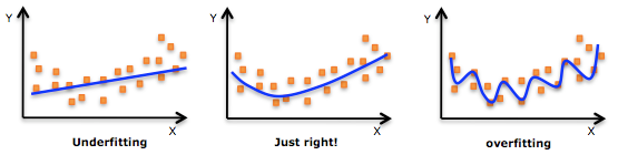
It is worth noting the underfitting is not as prevalent as overfitting. Nevertheless, we want to avoid both of those problems in data analysis. You might say we are trying to find the middle ground between under and overfitting our model. As you will see, train/test split and cross validation help to avoid overfitting more than underfitting. Let’s dive into both of them!

Train/Test Split

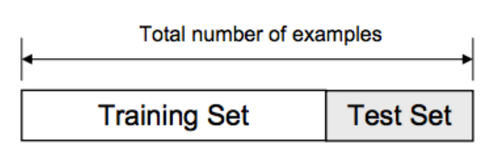
As I said before, the data we use is usually split into training data and test data. The training set contains a known output and the model learns on this data in order to be generalized to other data later on. We have the test dataset (or subset) in order to test our model’s prediction on this subset.

Let’s see how to do this in Python. We’ll do this using the Scikit-Learn library and specifically the train_test_split method. We’ll start with importing the necessary libraries:

import pandas as pd
from sklearn import datasets, linear_model
from sklearn.model_selection import train_test_split
from matplotlib import pyplot as plt

Let’s quickly go over the libraries I’ve imported:

Pandas — to load the data file as a Pandas data frame and analyze the data. If you want to read more on Pandas, feel free to
check out my post!
From Sklearn, I’ve imported the datasets module, so I can load a
sample dataset, and the linear_model, so I can run a linear
regression
From Sklearn, sub-library model_selection, I’ve imported the
train_test_split so I can, well, split to training and test sets
From Matplotlib I’ve imported pyplot in order to plot graphs of the
data

OK, all set! Let’s load in the diabetes dataset, turn it into a data frame and define the columns’ names:

# Load the Diabetes Housing dataset
columns = “age sex bmi map tc ldl hdl tch ltg glu”.split() # Declare the columns names
diabetes = datasets.load_diabetes() # Call the diabetes dataset from sklearn
df = pd.DataFrame(diabetes.data, columns=columns) # load the dataset as a pandas data frame
y = diabetes.target # define the target variable (dependent variable) as y

Now we can use the train_test_split function in order to make the split. The test_size=0.2 inside the function indicates the percentage of the data that should be held over for testing. It’s usually around 80/20 or 70/30.

# create training and testing vars
X_train, X_test, y_train, y_test = train_test_split(df, y, test_size=0.2)
print X_train.shape, y_train.shape
print X_test.shape, y_test.shape
(353, 10) (353,)
(89, 10) (89,)

Now we’ll fit the model on the training data:

# fit a model
lm = linear_model.LinearRegression()
model = lm.fit(X_train, y_train)
predictions = lm.predict(X_test)

As you can see, we’re fitting the model on the training data and trying to predict the test data. Let’s see what (some of) the predictions are:

predictions[0:5]
array([ 205.68012533,   64.58785513,  175.12880278,  169.95993301,128.92035866])

Note: because I used [0:5] after predictions, it only showed the first five predicted values. Removing the [0:5] would have made it print all of the predicted values that our model created.
Let’s plot the model:

## The line / model
plt.scatter(y_test, predictions)
plt.xlabel(“True Values”)
plt.ylabel(“Predictions”)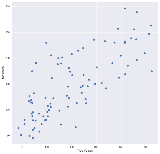

And print the accuracy score:

print “Score:”, model.score(X_test, y_test)
Score: 0.485829586737

There you go! Here is a summary of what I did: I’ve loaded in the data, split it into a training and testing sets, fitted a regression model to the training data, made predictions based on this data and tested the predictions on the test data. Seems good, right? But train/test split does have its dangers — what if the split we make isn’t random? What if one subset of our data has only people from a certain state, employees with a certain income level but not other income levels, only women or only people at a certain age? (imagine a file ordered by one of these). This will result in overfitting, even though we’re trying to avoid it! This is where cross validation comes in.

Cross Validation

In the previous paragraph, I mentioned the caveats in the train/test split method. In order to avoid this, we can perform something called cross validation. It’s very similar to train/test split, but it’s applied to more subsets. Meaning, we split our data into k subsets, and train on k-1 one of those subset. What we do is to hold the last subset for test. We’re able to do it for each of the subsets.

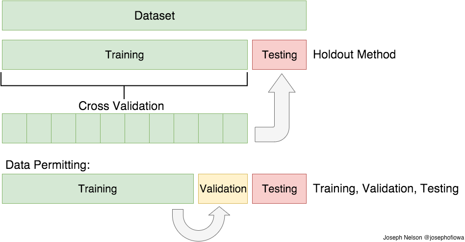
There are a bunch of cross validation methods, I’ll go over two of them: the first is K-Folds Cross Validation and the second is Leave One Out Cross Validation (LOOCV)

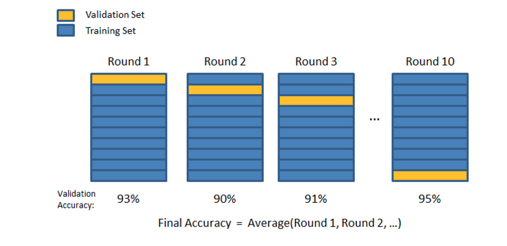
K-Folds Cross Validation

In K-Folds Cross Validation we split our data into k different subsets (or folds). We use k-1 subsets to train our data and leave the last subset (or the last fold) as test data. We then average the model against each of the folds and then finalize our model. After that we test it against the test set.

Here is a very simple example from the Sklearn documentation for K-Folds:

from sklearn.model_selection import KFold # import KFold
X = np.array([[1, 2], [3, 4], [1, 2], [3, 4]]) # create an array
y = np.array([1, 2, 3, 4]) # Create another array
kf = KFold(n_splits=2) # Define the split - into 2 folds
kf.get_n_splits(X) # returns the number of splitting iterations in the cross-validator
print(kf)
KFold(n_splits=2, random_state=None, shuffle=False)

And let’s see the result — the folds:

for train_index, test_index in kf.split(X):print(“TRAIN:”, train_index, “TEST:”, test_index)X_train, X_test = X[train_index], X[test_index]y_train, y_test = y[train_index], y[test_index]
('TRAIN:', array([2, 3]), 'TEST:', array([0, 1]))
('TRAIN:', array([0, 1]), 'TEST:', array([2, 3]))

As you can see, the function split the original data into different subsets of the data. Again, very simple example but I think it explains the concept pretty well.

Leave One Out Cross Validation (LOOCV)

This is another method for cross validation, Leave One Out Cross Validation (by the way, these methods are not the only two, there are a bunch of other methods for cross validation. Check them out in the Sklearn website). In this type of cross validation, the number of folds (subsets) equals to the number of observations we have in the dataset. We then average ALL of these folds and build our model with the average. We then test the model against the last fold. Because we would get a big number of training sets (equals to the number of samples), this method is very computationally expensive and should be used on small datasets. If the dataset is big, it would most likely be better to use a different method, like kfold.
Let’s check out another example from Sklearn:

from sklearn.model_selection import LeaveOneOut
X = np.array([[1, 2], [3, 4]])
y = np.array([1, 2])
loo = LeaveOneOut()
loo.get_n_splits(X)for train_index, test_index in loo.split(X):print("TRAIN:", train_index, "TEST:", test_index)X_train, X_test = X[train_index], X[test_index]y_train, y_test = y[train_index], y[test_index]print(X_train, X_test, y_train, y_test)

And this is the output:

('TRAIN:', array([1]), 'TEST:', array([0]))
(array([[3, 4]]), array([[1, 2]]), array([2]), array([1]))
('TRAIN:', array([0]), 'TEST:', array([1]))
(array([[1, 2]]), array([[3, 4]]), array([1]), array([2]))

Again, simple example, but I really do think it helps in understanding the basic concept of this method.
So, what method should we use? How many folds? Well, the more folds we have, we will be reducing the error due the bias but increasing the error due to variance; the computational price would go up too, obviously — the more folds you have, the longer it would take to compute it and you would need more memory. With a lower number of folds, we’re reducing the error due to variance, but the error due to bias would be bigger. It’s would also computationally cheaper. Therefore, in big datasets, k=3 is usually advised. In smaller datasets, as I’ve mentioned before, it’s best to use LOOCV.
Let’s check out the example I used before, this time with using cross validation. I’ll use the cross_val_predict function to return the predicted values for each data point when it’s in the testing slice.

# Necessary imports:
from sklearn.cross_validation import cross_val_score, cross_val_predict
from sklearn import metrics

As you remember, earlier on I’ve created the train/test split for the diabetes dataset and fitted a model. Let’s see what is the score after cross validation:

# Perform 6-fold cross validation
scores = cross_val_score(model, df, y, cv=6)
print “Cross-validated scores:”, scores
Cross-validated scores: [ 0.4554861   0.46138572  0.40094084  0.55220736  0.43942775  0.56923406]

As you can see, the last fold improved the score of the original model — from 0.485 to 0.569. Not an amazing result, but hey, we’ll take what we can get :)
Now, let’s plot the new predictions, after performing cross validation:

# Make cross validated predictions
predictions = cross_val_predict(model, df, y, cv=6)
plt.scatter(y, predictions)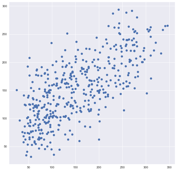

You can see it’s very different from the original plot from earlier. It is six times as many points as the original plot because I used cv=6.
Finally, let’s check the R² score of the model (R² is a “number that indicates the proportion of the variance in the dependent variable that is predictable from the independent variable(s)”. Basically, how accurate is our model):

accuracy = metrics.r2_score(y, predictions)
print “Cross-Predicted Accuracy:”, accuracy
Cross-Predicted Accuracy: 0.490806583864

That’s it for this time! I hope you enjoyed this post. As always, I welcome questions, notes, comments and requests for posts on topics you’d like to read. See you next time!

用Python进行训练/测试集分割和交叉验证相关推荐

python基于训练集预测_Python中训练集/测试集的分割和交叉验证
原标题:Python中训练集/测试集的分割和交叉验证嗨,大家好!在上一篇关于Python线性回归的文章之后,我认为撰写关于切分训练集/测试集和交叉验证的文章是很自然的,和往常一样,我将对该主题进行简 ...
标准化，归一化与训练-测试集数据处理
标准化,归一化与训练-测试集数据处理 1. 标准化,归一化的区别数据预处理的归一化手段应该如何应用到训练集,测试集和验证集中? 问题: 回答1: 回答2 问题3 回答1 回答2 问题4 回答1 1. ...
Keras训练神经网络进行分类并进行交叉验证（Cross Validation）
Keras训练神经网络进行分类并进行交叉验证(Cross Validation) 交叉验证是在机器学习建立模型和验证模型参数时常用的办法.交叉验证,顾名思义,就是重复的使用数据,把得到的样本数据进行切 ...
Python为给定模型执行留一法交叉验证实战LOOCV（leave-one-out cross-validation）
Python为给定模型执行留一法交叉验证实战LOOCV(leave-one-out cross-validation) 目录 Python为给定模型执行留一法交叉验证实战LOOCV(leave-one ...
Python计算医疗数据训练集、测试集的对应的临床特征：训练集（测试集）的阴性和阳性的样本个数、连续变量的均值（标准差）以及训练测试集阳性阴性的p值、离散变量的分类统计、比率、训练测试集阳性阴性的p值
Python使用pandas和scipy计算医疗数据训练集.测试集的对应的临床特征:训练集(测试集)的阴性和阳性的样本个数.连续变量的均值(标准差࿰
一文看懂 AI 训练集、验证集、测试集（附：分割方法+交叉验证）
2019-12-20 20:01:00 数据在人工智能技术里是非常重要的!本篇文章将详细给大家介绍3种数据集:训练集.验证集.测试集. 同时还会介绍如何更合理的讲数据划分为3种数据集.最后给大家介绍一 ...
python︱sklearn一些小技巧的记录（训练集划分/pipelline/交叉验证等）
sklearn里面包含内容太多,所以一些实用小技巧还是挺好用的. sklearn.cross_validation 如果没有了,则需要使用 sklearn.model_selection 文章目录 1 ...
label y 训练集测试集x_Adversarial validation-对抗验证| 一种解决训练集与测试集分布不一致的方法...
导语: 马上就要五一了,祝全世界人民五一快乐!在这之前,想过好几个准备这些天可以完成的专题,比如Boosting系列在搞点最近几年的新玩意,或者开一个新专题,如心心念念的GNN/GCN(主要是又可以去 ...
matlab 怎么求mape,如何有效地计算MATLAB中神经网络应用中训练/测试集的MAPE？
作为课程的一部分,我一直在使用MATLAB作为我的时间序列数据集(用于电数据集).它由40,000多个样本组成.神经网络形成后,我想测试它的准确性.我一直对MAPE(平均绝对误差)和RMS(均方根误差 ...

用Python进行训练/测试集分割和交叉验证