Naive Bayes: A classification algorithm under a supervised learning group based on Probabilistic logic. This is one of the simplest machine learning algorithms of all. Logistic regression is another classification algorithm that models posterior probability by learning input to output mapping and creates a discriminate model.

朴素贝叶斯(Naive Bayes)：一种基于概率逻辑的有监督学习小组下的分类算法。 这是所有最简单的机器学习算法之一。 Logistic回归是另一种分类算法，该算法通过学习输入到输出映射来建模后验概率并创建区分模型。

• Conditional Probability条件概率
• Independent events Vs. Mutually exclusive events独立事件与 互斥活动
• Bayes theorem with example贝叶斯定理与例子
• Naive Bayes Algorithm朴素贝叶斯算法
• Laplace smoothing拉普拉斯平滑
• Implementation of Naive Bayes Algorithm with Sci-kit learn朴素贝叶斯算法与Sci-kit学习的实现
• Pros & Cons优点缺点
• Summary摘要

Conditional Probability

条件概率

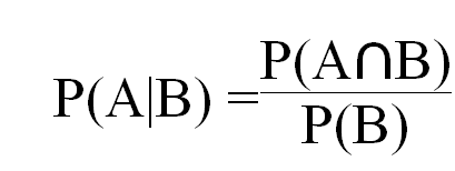
Conditional Probability is a measure of the probability of an event occurring given that another event has occurred.

条件概率是给定另一个事件已发生的情况下事件发生概率的度量。

Suppose, Ramesh wants to play cricket but he has to do his work, so there are two conditions first one is Ramesh wanna play cricket P(A) and the second one is he has to do his work P(B). So what is the probability that he can play cricket given that he already has a work P(A|B).

假设拉梅什想打板球，但他必须做他的工作，所以有两个条件，第一个条件是拉梅什想打板球P(A)，第二个条件是他必须做自己的工作P(B)。 那么，如果他已经有作品P(A | B)，那么他可以打板球的可能性是多少。

例如 ， (For example,)

Event A is drawing a Queen first, and Event B is drawing a Queen second.

事件A首先吸引女王，而事件B其次吸引女王。

For the first card the chance of drawing a Queen is 4 out of 52 (there are 4 Queens in a deck of 52 cards):

对于第一张牌，抽出一张女王的几率是52中的4(在52张牌中有4位皇后)：

P(A) = 4/52

P(A)= 4/52

But after removing a Queen from the deck the probability of the 2nd card drawn is less likely to be a Queen (only 3 of the 51 cards left are Queens):

但是，从卡组中移除女王后，第二张被抽出的可能性就不太可能是女王(剩下的51张卡中只有3张是女王)：

P(B|A) = 3/51

P(B | A)= 3/51

And so:

所以：

P(A⋂B) = P(A) x P(B|A) = (4/52) x (3/51) = 12/2652 = 1/221

P(A⋂B)= P(A)x P(B | A)=(4/52)x(3/51)= 12/2652 = 1/221

So the chance of getting 2 Queens is 1 in 221 or about 0.5%

因此，获得2个皇后的机会是221中的1个或约0.5％

Independent events Vs. Mutually exclusive events

独立事件与 互斥活动

P(A|B) is said to be Independent events if and only if events are occurring without affecting each other. Both events can occur simultaneously.

当且仅当事件发生而不相互影响时，才将P(A | B)称为独立事件。 这两个事件可以同时发生。

P(A|B) = P(A)

P(A | B)= P(A)

P(B|A)=P(B)

P(B | A)= P(B)

Let suppose there are two dies D1 and D2

假设有两个模具D1和D2

P(D1 = 6 | D2 = 3) = P(D1 =6)

P(D1 = 6 | D2 = 3)= P(D1 = 6)

Then there is no relationship between both two events occurrence. Both of the events are independent of each other.

这样，两个事件的发生之间就没有关系。 这两个事件彼此独立。

There is no impact of getting 6 on D1 to getting 3 on D2

在D1上获得6到D2上获得3的影响没有影响

Two events are mutually exclusive or disjoint if they cannot both occur at the same time.

如果两个事件不能同时发生，则它们是互斥或互斥的 。

Suppose,

假设，

The event is on D1 we wanna get 3 and same on the D1 we can’t get 5 because we already got 3 on D1.

该事件在D1上我们想要得到3，而在D1上我们同样不能得到5，因为我们已经在D1上得到3。

P(A|B)=P(B|A)=0

P(A | B)= P(B | A)= 0

P(A ∩ B) = P(B ∩ A) = 0

P(A∩B)= P(B∩A)= 0

It means both the events are cannot occur simultaneously.

这意味着两个事件不能同时发生。

Bayes Theorem with example

贝叶斯定理与例子

With this Image we can clearly see that the above given equation proved through the given steps.

借助此图像，我们可以清楚地看到上述给定的方程式已通过给定的步骤得到证明。

Suppose we have 3 machines A1,A2,A3 that produce an item given their probability & defective ratio.

假设我们有3台机器A1，A2，A3，根据它们的概率和次品率来生产一件物品。

p(A1) = 0.2

p(A1)= 0.2

p(A2) = 0.3

p(A2)= 0.3

p(A3) = 0.5

p(A3)= 0.5

B is representing defective

B代表缺陷

P(B|A1) = 0.05

P(B | A1)= 0.05

P(B|A2) = 0.03

P(B | A2)= 0.03

p(B|A3) = 0.01

p(B | A3)= 0.01

If an item is chosen as random then what is probability to be produced by Machine 3 given that item is defective (A3|B).

如果将某个项目选择为随机项目，则机器3假定该项目有缺陷(A3 | B)，那么该概率是多少。

P(B) = P (B|A1) P(A1) + P (B|A2) P(A2) +P (B|A3) P(A3)

P(B)= P(B | A1)P(A1)+ P(B | A2)P(A2)+ P(B | A3)P(A3)

P(B) = (0.05) (0.2) + (0.03) (0.3) + (0.01) (0.5)

P(B)=(0.05)(0.2)+(0.03)(0.3)+(0.01)(0.5)

P(B) = 0.024

P(B)= 0.024

Here 24% of the total Output of the factory is defective.

此处工厂总产量的24％有缺陷。

P(A3|B) = P(B|A3) P(A3)/P(B)

P(A3 | B)= P(B | A3)P(A3)/ P(B)

= (0.01) (0.50) / 0.024

=(0.01)(0.50)/ 0.024

= 5/24

= 5/24

= 0.21

= 0.21

Naive Bayes Algorithm

朴素贝叶斯算法

Given a vector x of features n where x is an independent variable

给定特征n的向量x ，其中x是自变量

C is classes.

C是类。

P( Ck | x1, x2, … xn )

P(Ck | x1，x2，…xn)

P( Ck | x) = (P(x | Ck) *P(Ck) ) / P(x)

P(Ck | x )=(P( x | Ck)* P(Ck))/ P( x )

Suppose given we are solving classification problem then we have to find two conditional probability P(C1|x) and P(C2|x). Out of these two binary classification probability which is highest we use that as maximum posterior.

假设给定我们正在解决分类问题，那么我们必须找到两个条件概率P(C1 | x)和P(C2 | x)。 在这两个最高的二元分类概率中，我们将其用作最大后验。

P(Ck ,x1 , x2, …, xn)=P(x1 , x2, …, xn,Ck )

P(Ck，x1，x2，...，xn)= P(x1，x2，...，xn，Ck)

which can be rewritten as follows, using the chain rule for repeated applications of the definition of conditional probability:

可以使用链式规则将其重写为条件概率定义的重复应用，如下所示：

P(x1 , x2, …, xn,Ck ) = P(x1 | x2, …, xn, Ck) * P(x2, …, xn, Ck)

P(x1，x2，...，xn，Ck)= P(x1 | x2，...，xn，Ck)* P(x2，...，xn，Ck)

= P(x1 | x2, …, xn, Ck) * P(x2, | x3, …, xn, Ck) * P(x3, …, xn, Ck)

= P(x1 | x2，…，xn，Ck)* P(x2，| x3，…，xn，Ck)* P(x3，…，xn，Ck)

= ….

=…。

= P(x1 | x2, …, xn, Ck) * P(x2, | x3, …, xn, Ck) * P(xn-1, | xn, Ck)* P(xn | Ck)* P(Ck)

= P(x1 | x2，…，xn，Ck)* P(x2，| x3，…，xn，Ck)* P(xn-1，| xn，Ck)* P(xn | Ck)* P(Ck )

Assume that all features in x are mutually independent, conditional on the category Ck

假设x中的所有要素都是相互独立的，且以类别Ck为条件

P(xi, | xi+1, …, xn, Ck) = P(xi, | Ck).

P(xi，| xi + 1，…，xn，Ck)＝ P(xi，| Ck)。

Thus, the joint model can be expressed as

因此，联合模型可以表示为

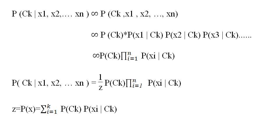
z is a scaling factor dependent only on x1,……xn that is, a constant if the values of the variables are known

z是仅取决于x1，…xn的比例因子，即，如果变量的值已知，则为常数

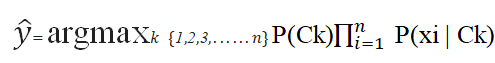
The discussion so far has derived the independent feature model, that is, the naive Bayes probability model. The naive Bayes classifier combines this model with a decision rule. One common rule is to pick the hypothesis that is most probable; this is known as the maximum a posterior or MAP decision rule. The corresponding classifier, a Bayes classifier, is the function that assigns a class label

到目前为止，讨论已经得出了独立的特征模型，即朴素的贝叶斯概率模型。 朴素的贝叶斯分类器将此模型与决策规则结合在一起。 一个普遍的规则是选择最可能的假设。 这称为最大后验或MAP决策规则。 相应的分类器(贝叶斯分类器)是分配类标签的函数

Example

例

Say you have 1000 fruits which could be either ‘banana’, ‘orange’ or ‘other’. These are the 3 possible classes of the Y variable.

假设您有1000种水果，可以是“香蕉”，“橙色”或“其他”。 这是Y变量的3种可能的类别。

We have data for the following X variables, all of which are binary (1 or 0).

我们具有以下X变量的数据，所有这些变量都是二进制的(1或0)。

• Long长
• Sweet甜
• Yellow黄色

The first few rows of the training dataset look like this:

训练数据集的前几行如下所示：

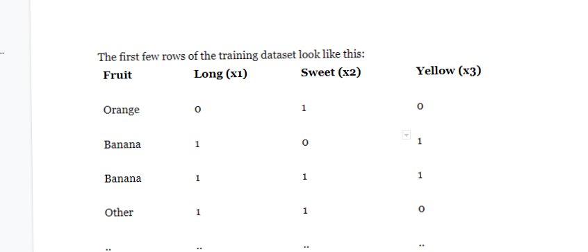
For the sake of computing the probabilities, let’s aggregate the training data to form a counts table like this.

为了计算概率，让我们汇总训练数据以形成这样的计数表。

So the objective of the classifier is to predict if a given fruit is a ‘Banana’ or ‘Orange’ or ‘Other’ when only the 3 features (long, sweet and yellow) are known.

因此，分类器的目的是在仅知道3个特征(长，甜和黄色)的情况下预测给定的水果是“香蕉”还是“橙色”或“其他”。

Let’s say you are given a fruit that is: Long, Sweet and Yellow, can you predict what fruit it is?

假设您得到的水果是：长，甜和黄色，您能预测它是什么水果吗？

This is the same of predicting the Y when only the X variables in testing data are known. Let’s solve it by hand using Naive Bayes.

这与仅知道测试数据中的X变量时预测Y相同。 让我们使用朴素贝叶斯解决它。

The idea is to compute the 3 probabilities, that is the probability of the fruit being a banana, orange or other. Whichever fruit type gets the highest probability wins.

这个想法是要计算3个概率，即水果是香蕉，橙子或其他的概率。 无论哪种水果获得最高的概率获胜。

All the information to calculate these probabilities is present in the above tabulation.

以上表格中列出了所有计算这些概率的信息。

Step 1: Compute the ‘Prior’ probabilities for each of the class of fruits.

步骤1：计算每种水果的“在先”概率。

That is, the proportion of each fruit class out of all the fruits from the population. You can provide the ‘Priors’ from prior information about the population. Otherwise, it can be computed from the training data.

也就是说，每种水果类别在人口中所有水果中所占的比例。 您可以从有关人口的先前信息中提供“优先”。 否则，可以根据训练数据进行计算。

For this case, let’s compute from the training data. Out of 1000 records in training data, you have 500 Bananas, 300 Oranges and 200 Others. So the respective priors are 0.5, 0.3 and 0.2.

对于这种情况，让我们根据训练数据进行计算。 在训练数据的1000条记录中，您有500个香蕉，300个橙子和200个其他。 因此，各个先验分别为0.5、0.3和0.2。

P(Y=Banana) = 500 / 1000 = 0.50

P(Y =香蕉)= 500/1000 = 0.50

P(Y=Orange) = 300 / 1000 = 0.30

P(Y =橙色)= 300/1000 = 0.30

P(Y=Other) = 200 / 1000 = 0.20

P(Y =其他)= 200/1000 = 0.20

Step 2: Compute the probability of evidence that goes in the denominator.

步骤2：计算进入分母的证据概率。

This is nothing but the product of P of Xs for all X. This is an optional step because the denominator is the same for all the classes and so will not affect the probabilities.

这不过是所有X的X的P的乘积。这是一个可选步骤，因为所有类的分母都相同，因此不会影响概率。

P(x1=Long) = 500 / 1000 = 0.50

P(x1 =长)= 500/1000 = 0.50

P(x2=Sweet) = 650 / 1000 = 0.65

P(x2 =甜)= 650/1000 = 0.65

P(x3=Yellow) = 800 / 1000 = 0.80

P(x3 =黄色)= 800/1000 = 0.80

Step 3: Compute the probability of likelihood of evidences that goes in the numerator.

步骤3：计算分子中证据出现的可能性。

It is the product of conditional probabilities of the 3 features. If you refer back to the formula, it says P(X1 |Y=k). Here X1 is ‘Long’ and k is ‘Banana’. That means the probability the fruit is ‘Long’ given that it is a Banana. In the above table, you have 500 Bananas. Out of that 400 is long. So, P(Long | Banana) = 400/500 = 0.8.

它是3个特征的条件概率的乘积。 如果回头看该公式，它将显示P(X1 | Y = k)。 X1是“长”，k是“香蕉”。 这意味着如果该水果是香蕉，则该水果“长”的概率。 在上表中，您有500个香蕉。 在这400个中很长。 因此，P(Long | Banana)= 400/500 = 0.8。

Here, I have done it for Banana alone.

在这里，我只为香蕉做过。

Probability of Likelihood for Banana

香蕉的可能性

P(x1=Long | Y=Banana) = 400 / 500 = 0.80

P(x1 =长| Y =香蕉)= 400/500 = 0.80

P(x2=Sweet | Y=Banana) = 350 / 500 = 0.70

P(x2 =甜| Y =香蕉)= 350/500 = 0.70

P(x3=Yellow | Y=Banana) = 450 / 500 = 0.90

P(x3 =黄色| Y =香蕉)= 450/500 = 0.90

So, the overall probability of Likelihood of evidence for Banana = 0.8 * 0.7 * 0.9 = 0.504

因此，香蕉证据的总体可能性为= 0.8 * 0.7 * 0.9 = 0.504

Step 4: Substitute all the 3 equations into the Naive Bayes formula, to get the probability that it is a banana.

步骤4：将所有三个方程式代入朴素贝叶斯公式，以得出它是香蕉的概率。

Similarly, you can compute the probabilities for ‘Orange’ and ‘Other fruit’. The denominator is the same for all 3 cases, so it’s optional to compute.

同样，您可以计算“橙色”和“其他水果”的概率。 这三种情况的分母都相同，因此计算是可选的。

Clearly, Banana gets the highest probability, so that will be our predicted class.

显然，香蕉获得的概率最高，因此这将是我们的预测类别。

Laplace Smoothing

拉普拉斯平滑

In statistics, Laplace Smoothing is a technique to smooth categorical data. Laplace Smoothing is introduced to solve the problem of zero probability. Laplace smoothing is used to deal with overfitting of models. Suppose in the given dataset if a word is not present at test time then we find out P(C=”Yes”|Textq) =0 or P(C=”No”|Textq).

在统计数据中，拉普拉斯平滑化是一种平滑分类数据的技术。 引入拉普拉斯平滑法来解决零概率问题。 拉普拉斯(Laplace)平滑用于处理模型的过拟合。 假设在给定的数据集中，如果单词在测试时不存在，那么我们找出P(C =“是” | Textq)= 0或P(C =“否” | Textq)。

Textq={w1,w2,w3,w4,W}

Textq = {w1，w2，w3，w4，W}

In the given training data we have w1,w2,w3 and w4 . But we don’t have W in training data so if we run P(C=”Yes”|Textq) or P(C=”No”|Textq) it we got

在给定的训练数据中，我们有w1，w2，w3和w4。 但是我们的训练数据中没有W，所以如果我们运行P(C =“是” | Textq)或P(C =“否” | Textq)，我们得到

P(C=”Yes”|Textq) =P(C=”No”|Textq)=0…………..condition (i)

P(C =“是” | Textq)= P(C =“否” | Textq)= 0…………..条件(i)

Because P(C=”Yes”|W) and P(C=”No”|W) we don’t have any probability value for this new word. So the value of probability is zero then ultimately our model is overfitting on train data because it can identify and classify the text which is available in the train data.

因为P(C =“是” | W)和P(C =“否” | W)，所以对于这个新单词我们没有任何概率值。 因此，概率值为零，则最终我们的模型对火车数据过度拟合，因为它可以识别和分类火车数据中可用的文本。

If the given dataset is imbalanced then the data model is underfitting and biased towards the majority class. To overcome this situation we use two different for binary classification and give more weightage to minor class to Balanced dataset.

如果给定的数据集不平衡，则数据模型不适合并且偏向多数类。 为了克服这种情况，我们对二进制分类使用两种不同的方法，并为“平衡”数据集的次要类赋予更大的权重。

P(C=”Yes”) we have λ1

P(C =“是”)我们有λ1

P(C=”No”) we have λ2 …………………… condition (ii)

P(C =“否”)我们有λ2……………………条件(ii)

To deal with this condition (i) and condition (ii) we used Laplace smoothing.

为了处理条件(i)和条件(ii)，我们使用了拉普拉斯平滑。

By applying this method, prior probability and conditional probability can be written as:

通过应用此方法，先验概率和条件概率可以写为：

K denotes the number of different values in y and A denotes the number of different values in aj. Usually lambda in the formula equals to 1.

K表示y中不同值的数量，而A表示aj中不同值的数量。 通常，公式中的lambda等于1。

By applying Laplace Smoothing, the prior probability and conditional probability in previous example can be written as:

通过应用拉普拉斯平滑，可以将前面示例中的先验概率和条件概率写为：

Here λ is a hyper-parameter to deal with Overfitting and Underfitting of models.

λ是一个超参数，用于处理模型的过拟合和欠拟合。

When the value of λ Decreasing that time model is Overfitting because it gives less value to the new word or imbalance data.

当“减少时间”的“λ值”为“过拟合”时，因为它给新单词或不平衡数据赋予的值较小。

When the value of λ Increasing that time model is Underfitting.

当“增加该时间”的“λ”值是“拟合不足”时。

λ is used for tug-of-bar between Overfitting and Underfitting of models.

λ用于模型的过拟合和欠拟合之间的拔河。

Implementation of Naive Bayes in Sci-kit learn

在Sci-kit中实施朴素贝叶斯学习

Applications of Naive Bayes Algorithm

朴素贝叶斯算法的应用

1. Real-time Prediction: As Naive Bayes is super fast, it can be used for making predictions in real time.

   实时预测 ：由于朴素贝叶斯非常快，因此可以用于实时预测。

2. Multi-class Prediction: This algorithm can predict the posterior probability of multiple classes of the target variable.

   多类预测 ：该算法可以预测目标变量的多类后验概率。

3. Text classification/ Spam Filtering/ Sentiment Analysis: Naive Bayes classifiers are mostly used in text classification (due to their better results in multi-class problems and independence rule) have a higher success rate as compared to other algorithms. As a result, it is widely used in Spam filtering (identify spam email) and Sentiment Analysis (in social media analysis, to identify positive and negative customer sentiments)

   文本分类/垃圾邮件过滤/情感分析 ：朴素贝叶斯分类器主要用于文本分类(由于它们在多类问题和独立性规则方面的更好结果)与其他算法相比具有较高的成功率。 因此，它被广泛用于垃圾邮件过滤(识别垃圾邮件)和情感分析(在社交媒体分析中，确定正面和负面的客户情绪)

4. Recommendation System: Naive Bayes Classifier along with algorithms like Collaborative Filtering makes a Recommendation System that uses machine learning and data mining techniques to filter unseen information and predict whether a user would like a given resource or not.

   推荐系统 ：朴素贝叶斯分类器与诸如协同过滤之类的算法一起构成了一个推荐系统，该推荐系统使用机器学习和数据挖掘技术来过滤看不见的信息并预测用户是否希望使用给定资源。

优点缺点 (Pros &Cons)

Pros:

优点：

• It is easy and fast to predict the class of test data sets. It also perform well in multi class prediction预测测试数据集的类别既容易又快速。 在多类别预测中也表现出色
• When assumption of independence holds, a Naive Bayes classifier performs better compared to other models like logistic regression and you need less training data.如果保持独立性假设，那么与其他模型(例如逻辑回归)相比，朴素贝叶斯分类器的性能会更好，并且您需要的训练数据也更少。
• It performs well in case of categorical input variables compared to numerical variable(s). For numerical variables, Gaussian normal distribution is assumed (bell curve, which is a strong assumption).与数字变量相比，在分类输入变量的情况下，它表现良好。 对于数值变量，假定为高斯正态分布(钟形曲线，这是一个很强的假设)。

Cons:

缺点：

• If a categorical variable has a category (in test data set), which was not observed in training data set, then the model will assign a 0 (zero) probability and will be unable to make a prediction. This is often known as “Zero Frequency”. To solve this, we can use the smoothing technique. One of the simplest smoothing techniques is called Laplace estimation.如果分类变量具有一个类别(在测试数据集中)，而该类别在训练数据集中没有被观察到，则该模型将分配0(零)概率，并且将无法进行预测。 这通常被称为“零频率”。 为了解决这个问题，我们可以使用平滑技术。 最简单的平滑技术之一称为拉普拉斯估计。
• On the other side naive Bayes is also known as a bad estimator, so the probability outputs from predict_proba are not to be taken too seriously.另一方面，朴素的贝叶斯也被认为是一个不好的估计量，因此，predict_proba的概率输出不要太当真。
• Another limitation of Naive Bayes is the assumption of independent predictors. In real life, it is almost impossible that we get a set of predictors which are completely independent.朴素贝叶斯的另一个局限性是独立预测变量的假设。 在现实生活中，我们几乎不可能获得一组完全独立的预测变量。

Summary

摘要

In this Blog, you will learn about What is Conditional Probability and Different types of events that are used in Bayes theorem.

在此博客中，您将了解什么是条件概率和贝叶斯定理中使用的不同类型的事件。

How Bayes theorem is applied in Naive Bayes Algorithm.

朴素贝叶斯算法如何应用贝叶斯定理。

How Naive Bayes algorithm deals with Overfitting and Underfitting.

朴素贝叶斯算法如何处理过拟合和欠拟合。

How to Implement algorithm with sci-kit learn.

如何使用sci-kit学习实现算法。

What are the application of Naive Bayes Algorithm.

朴素贝叶斯算法有哪些应用。

What is Procs & Cons of algorithm.

什么是算法的过程与缺点。