A Monte Carlo Markov Chain (MCMC) is a model describing a sequence of possible events where the probability of each event depends only on the state attained in the previous event. MCMC have a wide array of applications, the most common of which is the approximation of probability distributions.

蒙特卡洛马尔可夫链 ( MCMC )是描述一系列可能事件的模型，其中每个事件的概率仅取决于先前事件中达到的状态。 MCMC具有广泛的应用，其中最常见的是概率分布的近似值。

Let’s take a look at an example of Monte Carlo Markov Chains in action. Suppose we wanted to determine the probability of sunny (S) and rainy (R) weather.

让我们看一下蒙特卡洛·马尔科夫链的实际例子。 假设我们要确定晴天(S)和多雨(R)的概率。

We’re given the following conditional probabilities:

我们得到以下条件概率：

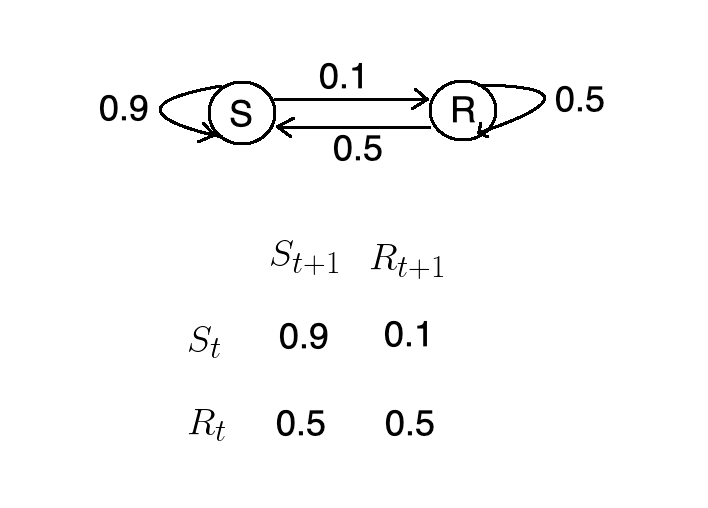
• If it’s rainy today, there’s a 50% chance that it will be sunny tomorrow.如果今天下雨，明天有50％的可能性是晴天。
• If it’s rainy today, there’s a 50% chance it will be raining tomorrow.如果今天下雨，明天有50％的机会会下雨。
• If it’s sunny today, there’s a 90% chance it will be sunny tomorrow.如果今天天气晴朗，则明天有90％的机会会晴天。
• If it’s sunny today, there’s a 10% chance it will be raining tomorrow.如果今天晴天，明天有10％的机会会下雨。

Let’s assume we started out in the sunny state. We then do a Monte Carlo simulation. That is to say, we generate a random number between 0 and 1, and if it happens to be below 0.9, it will be sunny tomorrow, and rainy otherwise. We do another Monte Carlo simulation, and this time around, it’s going to be rainy tomorrow. We repeat the process for n iterations.

假设我们从阳光明媚的状态开始。 然后，我们进行蒙特卡洛模拟。 也就是说，我们生成一个介于0和1之间的随机数，如果它恰好低于0.9，则明天将是晴天，否则将下雨。 我们再进行一次蒙特卡洛模拟，这一次，明天会下雨。 我们重复此过程n次迭代。

The following sequence is known as a Markov Chain.

以下序列称为马尔可夫链。

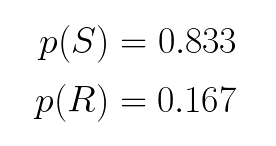
We count the number of sunny days and divide by the total number of days to determine the probability that it will be sunny. If the Markov Chain are long enough, even though the initial states might be different, we will obtain the same marginal probability. In this case, the probability that it will be sunny is 83.3%, and the probability that it will be rainy is 16.7%.

我们计算晴天的次数，然后除以总天数，以确定晴天的概率。 如果马尔可夫链足够长，即使初始状态可能不同，我们将获得相同的边际概率。 在这种情况下，晴天的概率是83.3％，而下雨的概率是16.7％。

Let’s see how we might go about implementing a Monte Carlo Markov Chain in Python.

让我们看看如何在Python中实现蒙特卡洛马尔可夫链。

We begin by importing the following libraries:

我们首先导入以下库：

import numpy as npfrom matplotlib import pyplot as pltimport seaborn as snssns.set()

We can express the conditional probabilities from the previous example using a state machine, and corresponding matrix.

我们可以使用状态机和相应的矩阵来表达上一个示例中的条件概率。

We perform some linear algebra.

我们执行一些线性代数。

T = np.array([[0.9, 0.1],[0.5, 0.5]])p = np.random.uniform(low=0, high=1, size=2)p = p/np.sum(p)q=np.zeros((100,2))for i in np.arange(0,100):    q[i, :] = np.dot(p,np.linalg.matrix_power(T, i))

Finally, we plot the results.

最后，我们绘制结果。

plt.plot(q)plt.xlabel('i')plt.legend(('S', 'R'))

As we can see, the probability that it will be sunny settles around 0.833. Similarly, the probability that it will be rainy converges towards 0.167.

如我们所见，晴天的概率大约为0.833。 同样，下雨的可能性收敛至0.167。

贝叶斯公式 (Bayes Formula)

Often times, we want to know the probability of some event, given that another event has occurred. This can be expressed symbolically as p(B|A). If two events are not independent then the probability of both occurring is expressed by the following formula.

通常，我们想知道某个事件的发生概率，因为发生了另一个事件。 这可以象征性地表示为p(B | A) 。 如果两个事件不是独立的，则两个事件发生的可能性由以下公式表示。

For example, suppose we are drawing two cards from a standard deck of 52 cards. Half of all cards in the deck are red and half are black. These events are not independent because the probability of the second draw depends on the first.

例如，假设我们从52张标准牌中抽取了2张牌。 卡组中所有卡的一半是红色，一半是黑色。 这些事件不是独立的，因为第二次抽奖的概率取决于第一次。

P(A) = P(black card on first draw) = 25/52 = 0.5

P(A)= P(首次抽奖时黑牌)= 25/52 = 0.5

P(B|A) = P(black card on second draw | black card on first draw) = 25/51 = 0.49

P(B | A)= P(第二次抽奖中的黑卡|第一次抽奖中的黑卡)= 25/51 = 0.49

Using this information, we can calculate the probability of drawing two black cards in a row as:

使用此信息，我们可以计算出连续绘制两张黑卡的概率为：

Now, let’s suppose that instead, we wanted to develop a spam filter that will categorize an email as spam or not depending on the occurrence of some word. For example, if an email contains the word Viagra, we classify it as spam. If on the other hand, an email contains the word money, then there’s an 80% chance that it’s spam.

现在，让我们假设，我们想要开发一个垃圾邮件过滤器，该过滤器将根据某些单词的出现将电子邮件归类为垃圾邮件。 例如，如果电子邮件中包含“ 伟哥 ”一词，我们会将其分类为垃圾邮件。 另一方面，如果电子邮件中包含金钱一词，则有80％的可能性是垃圾邮件。

According to Bayes Theorem, the probability that an email is spam given that it contains a given word is:

根据贝叶斯定理，假设电子邮件包含给定单词，则该电子邮件为垃圾邮件的可能性为：

We might know the probability that an email is spam as well as the probability that a word is contained in an email classified as spam. We do not, however, know the probability that a given word will be found in an email. This is where the Metropolis-Hastings algorithm come in to play.

我们可能知道电子邮件为垃圾邮件的可能性，以及包含在归类为垃圾邮件的电子邮件中的单词的可能性。 但是，我们不知道在电子邮件中找到给定单词的可能性。 这是Metropolis-Hastings算法发挥作用的地方。

Metropolis Hastings算法 (Metropolis Hastings Algorithm)

The Metropolis-Hasting algorithm enables us to determine the posterior probability without knowing the normalizing constant. At a high level, the Metropolis-Hasting algorithm works as follows:

Metropolis-Hasting算法使我们能够确定后验概率，而无需知道归一化常数。 在较高级别，Metropolis-Hasting算法的工作原理如下：

The acceptance criteria only looks at ratios of the target distribution, so the denominator cancels out.

接受标准仅考虑目标分布的比率，因此分母会抵消。

For you visual learners out there, let’s illustrate how the algorithm works with an example.

对于在那里的视觉学习者，让我们通过一个示例来说明该算法的工作原理。

We begin by selecting a random initial value for theta.

我们从为theta选择一个随机初始值开始。

Then, we propose a new value for theta.

然后，我们提出theta的新值。

We calculate the ratio of the PDF at current value of theta and the PDF at the proposed value of theta.

我们计算了当前值theta时PDF与建议值theta时PDF的比率。

If rho is less than 1, then we set theta to the new value with probability p. We do so by comparing rho with a sample u drawn from a uniform distribution. If rho is greater than u then we accept the proposed value, otherwise, we reject it.

如果rho小于1，则将theta设置为概率为p的新值。 我们通过与ü从均匀分布中抽取的样本比较RHO这样做。 如果rho大于u，则我们接受建议的值，否则，我们拒绝它。

We try a different value for theta.

我们尝试使用不同的theta值。

If rho is greater than 1 it will always be greater or equal to the sample drawn from the uniform distribution. Thus, we accept the proposal for the new value of theta.

如果rho大于1，它将始终大于或等于从均匀分布中提取的样本。 因此，我们接受有关theta新值的提议。

We repeat the process n number of iterations.

我们重复n次迭代。

Since we automatically accept a proposed move when the target distribution is greater than the one at the current position, theta will tend to be in places where the target distribution is denser. However, if we only accepted values that were greater than the current position, we’d get stuck at one of the peaks. Therefore, we occasionally accept moves to lower density regions. This way, theta will be expected to bounce around in such a way as to approximate the density of the posterior distribution.

由于当目标分布大于当前位置的目标位置时，我们会自动接受建议的移动，因此theta往往位于目标分布较密集的地方。 但是，如果我们只接受大于当前位置的值，则将卡在其中一个峰上。 因此，我们偶尔会接受向较低密度区域移动。 这样，将期望θ以近似后验分布的密度的方式反弹。

The sequence of steps is in fact a Markov Chain.

步骤的顺序实际上是马尔可夫链。

Let’s walk through how we’d go about implemented the Metropolis-Hasting algorithm in Python, but first, here’s a quick refresher on the different types of distributions.

让我们逐步介绍如何在Python中实现Metropolis-Hasting算法，但首先，这里是有关不同类型发行版的快速复习。

正态分布 (Normal Distribution)

In nature random phenomenon (i.e. IQ, height) tend to follow a normal distribution. A normal distribution has two parameters Mu, and Sigma. Varying Mu shifts the bell curve, whereas varying Sigma alters the width of the bell curve.

在自然界中，随机现象(即智商，身高)倾向于遵循正态分布。 正态分布具有两个参数Mu和Sigma。 改变Mu会改变钟形曲线，而改变Sigma会改变钟形曲线的宽度。

Beta分布 (Beta Distribution)

Like a normal distribution, beta distribution has two parameters. However, unlike a normal distribution, the shape of a beta distribution will vary significantly based on the values of its parameters alpha and beta.

像正态分布一样，β分布具有两个参数。 但是，与正态分布不同，β分布的形状将基于其参数alpha和beta的值而显着变化。

二项分布 (Binomial Distribution)

Unlike a normal distribution that could have height as its domain, the domain of a binomial distribution will always be the number of discrete events.

与正态分布可能以高度为域不同，二项分布的域始终是离散事件的数量。

Now that we’ve familiarized ourselves with these concepts, we’re ready to delve into the code. We begin by initializing the hyperparameters.

现在我们已经熟悉了这些概念，我们准备深入研究代码。 我们首先初始化超参数。

n = 100h = 59a = 10b = 10sigma = 0.3theta = 0.1niters = 10000thetas = np.linspace(0, 1, 200)samples = np.zeros(niters+1)samples[0] = theta

Next, we define a function that will return the multiplication of the likelihood and prior for a given value of theta.

接下来，我们定义一个函数，该函数将为给定的theta值返回似然和先验的乘积。

def prob(theta):    if theta < 0 or theta > 1:        return 0    else:        prior = st.beta(a, b).pdf(theta)        likelihood = st.binom(n, theta).pmf(h)        return likelihood * prior

We step through the algorithm updating the values of theta based off the conditions described earlier.

我们逐步执行基于前面所述条件更新theta值的算法。

for i in range(niters):    theta_p = theta + st.norm(0, sigma).rvs()    rho = min(1, prob(theta_p) / prob(theta))    u = np.random.uniform()    if u < rho:        # Accept proposal        theta = theta_p    else:        # Reject proposal        pass    samples[i+1] = theta

We define the likelihood, as well as the prior and post probability distributions.

我们定义可能性，以及先后概率分布。

prior = st.beta(a, b).pdf(thetas)post = st.beta(h+a, n-h+b).pdf(thetas)likelihood = st.binom(n, thetas).pmf(h)

We visualize the posterior distribution obtained using the Metropolis-Hastings algorithm.

我们可视化使用Metropolis-Hastings算法获得的后验分布。

plt.figure(figsize=(12, 9))plt.hist(samples[len(samples)//2:], 40, histtype='step', normed=True, linewidth=1, label='Predicted Posterior');plt.plot(thetas, n*likelihood, label='Likelihood', c='green')plt.plot(thetas, prior, label='Prior', c='blue')plt.plot(thetas, post, c='red', linestyle='--', alpha=0.5, label='True Posterior')plt.xlim([0,1]);plt.legend(loc='best');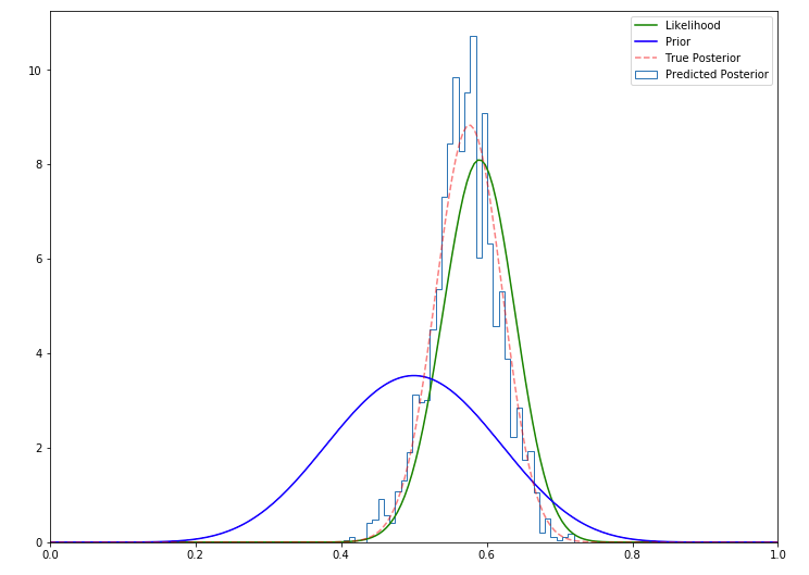

As we can see, the Metropolis Hasting method does a good job of approximating the actual posterior distribution.

如我们所见，Metropolis Hasting方法在逼近实际后验分布方面做得很好。

结论 (Conclusion)

A Monte Carlo Markov Chain is a sequence of events drawn from a set of probability distributions that can be used to approximate another distribution. The Metropolis-Hasting algorithm makes use of Monte Carlo Markov Chains to approximate the posterior distribution when we know the likelihood and prior, but not the normalizing constant.

蒙特卡洛马尔可夫链是从一系列概率分布中得出的事件序列，可用于近似另一个分布。 当我们知道似然和先验但不知道归一化常数时，Metropolis-Hasting算法利用蒙特卡洛马尔可夫链来近似后验分布。