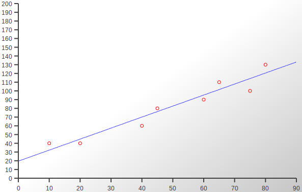
In a previous post I implemented the Pearson Correlation Coefficient, a measure of how much one variable depends on another. The three sets of bivariate data I used for testing and demonstration are shown again below, along with their corresponding scatterplots. As you can see these scatterplots now have lines of best fit added, their gradients and heights being calculated using least-squares regression which is the subject of this article.

在上一篇文章中，我实现了Pearson相关系数，它是一个变量对另一个变量的依赖程度的度量。 下面再次显示了我用于测试和演示的三组双变量数据及其对应的散点图。 如您所见，这些散点图现在添加了最合适的线，它们的梯度和高度是使用最小二乘回归计算的，这是本文的主题。

数据集1 (Data Set 1)

数据集2 (Data Set 2)

数据集3 (Data Set 3)

线性方程y = ax + b (The Linear Equation y = ax + b)

To draw the line of best fit we need the two end points which are then just joined up. The values of x are between 0 and 90 so if we have a formula in the form

为了画出最合适的线，我们需要将两个端点连接起来。 x的值在0到90之间，所以如果我们有一个形式为

y = ax + b

y = ax + b

we can then plug in 0 and 90 as the values of x to get the corresponding values for y.

然后，我们可以插入0和90作为x的值，以获得y的相应值。

a represents the gradient or slope of the line, for example if y increases at the same rate as x then a will be 1, if it increases at twice the rate then a will be 2 etc. (The x and y axes might be to different scales in which case the apparent gradient might not be the same as the actual gradient.) b is the offset, or the amount the line is shifted up or down. If the scatterplot’s x-axis starts at or passes through 0 then the height of the line at that point will be the same as b.

a表示直线的斜率或斜率，例如，如果y以与x相同的速率增加，则a将为1，如果y以两倍的速率增加，则a将为2，依此类推。( x和y轴可能是不同的比例，在这种情况下，视在渐变可能与实际渐变不同。) b是偏移量，或直线上移或下移的量。 如果散点图的x轴从0开始或经过0，则该点处的线的高度将与b相同。

I have used the equation of the line in the form ax + b, but mx + c is also commonly used. Also, the offset is sometimes put first, ie. b + ax or c + mx.

我以ax + b的形式使用了直线方程，但是mx + c也很常用。 另外，有时会将偏移量放在第一位。 b + ax或c + mx 。

插值和外推 (Interpolation and Extrapolation)

Apart from drawing a line to give an immediate and intuitive impression of the relationship between two variables, the equation given by linear or other kinds of regression can also be used to estimate values of y for values of x either within or outside the known range of values.

除了画一条线以直观地直观了解两个变量之间的关系外，线性或其他类型的回归方程还可以用于估计x值在已知范围内或之外的y值。价值观。

Estimating values within the current range of the independent variable is known as interpolation, for example in Data Set 1 we have no data for x = 30, but once we have calculated a and b we can use them to calculate an estimated value of y for x = 30.

估计自变量当前范围内的值称为插值，例如，在数据集1中，没有x = 30的数据，但是一旦我们计算了a和b，就可以使用它们来计算y的估计值x = 30。

The related process of estimating values outside the range of known x values (in these examples < 0 and > 90) is known as extrapolation.

估计已知x值范围之外的值(在这些示例中<0和> 90)之外的相关过程称为外推法。

The results of interpolation and extrapolation need to be treated with caution. Even if the known data fits a line exactly does not imply that unknown values will also fit, and of course the more imperfect the fit the more unlikely unknown values are to be on or near the regression line.

内插和外推的结果需要谨慎对待。 即使已知数据完全符合一条线，也并不意味着未知值也将符合，当然，拟合越不完美，未知值出现在回归线上或接近回归线的可能性就越小。

One reason for this is a limited set of data which might not be representative of all possible data. Another is that the range of independent variables might be small, fitting a straight line within a limited range but actually following a more complex pattern over a wider range of values.

这样做的一个原因是有限的数据集，可能不能代表所有可能的数据。 另一个是自变量的范围可能很小，在有限的范围内拟合一条直线，但实际上在更宽的值范围内遵循更复杂的模式。

As an example, imagine temperature data for a short period during spring. It might appear to rise linearly during this period, but of course we know it will level out in summer before dropping off through winter, before repeating an annual cycle. A linear model for such data is clearly useless for extrapolation.

例如，想象一下SpringSpring的短期温度数据。 在此期间，它似乎呈线性上升，但我们当然知道，它将在夏季趋于平稳，然后在整个冬季下降，然后再重复年度周期。 此类数据的线性模型显然无法进行推断。

回归是AI吗？ (Is Regression AI?)

The concept of regression discussed here goes back to the early 19th Century, when of course it was calculated by hand using pencil and paper. Therefore the answer to the question “is it artificial intelligence” is obviously “don’t be stupid, of course it isn’t!”

这里讨论的回归概念可以追溯到19世纪初，当时当然是用铅笔和纸手工计算出来的。 因此，“是否是人工智能”问题的答案显然是“不要傻，当然不是！”

The term artificial intelligence has been around since 1956, and existed as a serious idea (ie. beyond just sci-fi or fantasy) since the 1930s when Alan Turing envisaged computers as more brain-like in their functionality than actually happened. The idea that for decades computers would be little more than calculators or filing systems would not have impressed him. This is perhaps longer than many people imagine but still nowhere near as far back as the early 1800s.

人工智能一词始于1956年，自1930年代开始就以一个严肃的想法存在(即，不仅是科幻或幻想)，当时艾伦·图灵(Alan Turing)设想计算机的功能要比实际发生的更像大脑。 几十年来，计算机只不过是计算器或文件系统的想法并没有给他留下深刻的印象。 这可能比许多人想象的要长，但仍远不及1800年代初期。

AI has had a chequered history, full of false starts, dead ends and disappointments, and has only started to become mainstream and actually useful in the past few years. This is due mainly to the emergence of machine learning, so AI and ML are sometimes now being used interchangeably.

人工智能历史悠久，充满了错误的开始，死胡同和失望，并且在过去的几年中才开始成为主流并真正有用。 这主要是由于机器学习的出现，因此AI和ML现在有时可以互换使用。

The existence of very large amounts of data (“Big Data”) plus the computing power to crunch that data using what are actually very simple algorithms has led to this revolution. With enough data and computing power you can derive generalised rules (ie. numbers) from samples which can be used to make inferences or decisions on other, similar, items of data.

大量数据(“大数据”)的存在以及使用实际上非常简单的算法处理数据的计算能力导致了这场革命。 有了足够的数据和计算能力，您就可以从样本中得出通用规则(即数字)，这些规则可用于对其他类似数据项进行推断或决策。

Hopefully you can see what I am getting at here: carry out regression on the data you have, then use the results for interpolation and extrapolation about other possible data — almost a definition of Machine Learning.

希望您能看到我在这里得到的结果：对您拥有的数据进行回归，然后将结果用于其他可能数据的内插和外推-几乎是机器学习的定义。

编写代码 (Writing the Code)

For this project we will write the code necessary to carry out linear regression, ie. calculate a and b, and then write a method to create sample lists of data corresponding to that shown above for testing and demonstrating the code.

对于此项目，我们将编写执行线性回归所需的代码，即。 计算a和b ，然后编写一种方法来创建与上面显示的数据相对应的数据示例列表，以测试和演示代码。

The project consists of these files which you can clone or download from the Github repository:

该项目包含以下文件，您可以从Github存储库中克隆或下载这些文件：

• linearregression.py线性回归
• data.pydata.py
• main.pymain.py

Lets’s first look at linearregression.py.

首先让我们看一下linearregression.py 。

import mathclass LinearRegression(object):"""Implements linear regression on two lists of numericsSimply set independent_data and dependent_data,call the calculate method,and retrieve a and b"""def __init__(self):"""Not much happening here - just create empty attributes"""self.independent_data = Noneself.dependent_data = Noneself.a = Noneself.b = Nonedef calculate(self):"""After calling separate functions to calculate a few intermediate valuescalculate a and b (gradient and offset)."""independent_mean = self.__arithmetic_mean(self.independent_data)dependent_mean = self.__arithmetic_mean(self.dependent_data)products_mean = self.__mean_of_products(self.independent_data, self.dependent_data)independent_variance = self.__variance(self.independent_data)self.a = (products_mean - (independent_mean * dependent_mean) ) / independent_varianceself.b = dependent_mean - (self.a * independent_mean)def __arithmetic_mean(self, data):"""The arithmetic mean is what most people refer to as the "average",or the total divided by the count"""total = 0for d in data:total += dreturn total / len(data)def __mean_of_products(self, data1, data2):"""This is a type of arithmetic mean, but of the products of corresponding valuesin bivariate data"""total = 0for i in range(0, len(data1)):total += (data1[i] * data2[i])return total / len(data1)def __variance(self, data):"""The variance is a measure of how much individual items of data typically vary from themean of all the data.The items are squared to eliminate negatives.(The square root of the variance is the standard deviation.)"""squares = []for d in data:squares.append(d**2)mean_of_squares = self.__arithmetic_mean(squares)mean_of_data = self.__arithmetic_mean(data)square_of_mean = mean_of_data**2variance = mean_of_squares - square_of_meanreturn variance

The __init__ method just creates a few default values. The calculate method is central to this project as it actually calculates a and b. To do this it needs a few intermediate variables: the means of the two sets of data, the mean of the products of the corresponding data items, and the variance. These are all calculated by separate functions. Finally we calculate a and b using the formulae which should be clear from the code.

__init__方法仅创建一些默认值。 该calculate方法对该项目非常重要，因为它实际上计算a和b 。 为此，它需要一些中间变量：两组数据的平均值，相应数据项乘积的平均值以及方差。 这些都是由单独的函数计算的。 最后，我们使用应该从代码中清楚看出的公式来计算a和b 。

The arithmetic mean is what most people think of as the average, ie the total divided by the count.

算术平均值是大多数人认为的平均值，即总数除以计数。

The mean of products is also an arithmetic mean, but of the products of each pair of values.

乘积的平均值也是算术平均值，但是是每对值的乘积。

The variance is, as I have described in the docstring, “a measure of how much individual items of data typically vary from the mean of all the data”.

如我在文档字符串中所述，方差是“衡量单个数据项通常与所有数据均值之间的差异的度量”。

Now let’s move on to data.py.

现在让我们进入data.py。

def populatedata(independent, dependent, dataset):"""Populates the lists with one of three datasets suitablefor demonstrating linear regression code"""del independent[:]del dependent[:]if dataset == 1:independent.extend([10,20,40,45,60,65,75,80])dependent.extend([32,44,68,74,92,98,110,116])return Trueelif dataset == 2:independent.extend([10,20,40,45,60,65,75,80])dependent.extend([40,40,60,80,90,110,100,130])return Trueelif dataset == 3:independent.extend([10,20,40,45,60,65,75,80])dependent.extend([100,10,130,90,40,80,180,50])return Trueelse:return False

The populatedata method takes two lists and, after emptying them just in case they are being reused, adds one of the three pairs of datasets listed earlier.

populatedata方法采用两个列表，在清空它们以防万一它们被重用之后，添加前面列出的三对数据集之一。

Now we can move on to the main function and put the above code to use.

现在我们可以转到main函数并使用上面的代码。

import data
import linearregressiondef main():"""Demonstrate the LinearRegression class with three sets of test dataprovided by the data module"""print("---------------------")print("| codedrome.com     |")print("| Linear Regression |")print("---------------------\n")independent = []dependent = []lr = linearregression.LinearRegression()for d in range(1, 4):if data.populatedata(independent, dependent, d) == True:lr.independent_data = independentlr.dependent_data = dependentlr.calculate()print("Dataset %d\n---------" % d)print("Independent data: " + (str(lr.independent_data)))print("Dependent data:   " + (str(lr.dependent_data)))print("y = %gx + %g" % (lr.a, lr.b))print("")else:print("Cannot populate Dataset %d" % d)main()

Firstly we create a pair of empty lists and a LinearRegression object. Then in a loop we call populatedata and set the LinearRegression object’s data lists to the local lists. Next we call the calculate method and print the results.

首先，我们创建一对空列表和一个LinearRegression对象。 然后在一个循环中，我们调用populatedata ，并将LinearRegression对象的数据列表设置为本地列表。 接下来，我们调用calculate方法并打印结果。

That’s the code finished so we can run it with the following in Terminal:

代码已完成，因此我们可以在Terminal中使用以下代码运行它：

python3.8 main.py

python3.8 main.py

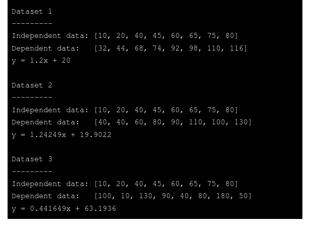
The program output shows each of the three sets of data, along with the formulae of their respective lines of best fit.

程序输出显示三组数据中的每组数据，以及各自最佳拟合线的公式。

In the section above on interpolation and extrapolation, I used x = 30 in Data Set 1 as an example of missing data which could be estimated by interpolation. Now we have values of a and b for that data we can use them as follows:

在上面有关内插和外推的部分中，我以数据集1中的x = 30为例，可以通过内插来估计丢失的数据。 现在我们对该数据有了a和b值，可以按以下方式使用它们：