Hough transform

From Wikipedia, the free encyclopedia

The Hough transform (pronounced /ˈhʌf/ to rhyme with rough) is a feature extraction technique used in image analysis, computer vision, and digital image processing.^[1] The purpose of the technique is to find imperfect instances of objects within a certain class of shapes by a voting procedure. This voting procedure is carried out in a parameter space, from which object candidates are obtained as local maxima in a so-called accumulator space that is explicitly constructed by the algorithm for computing the Hough transform.

The classical Hough transform was concerned with the identification of lines in the image, but later the Hough transform has been extended to identifying positions of arbitrary shapes, most commonly circles or ellipses. The Hough transform as it is universally used today was invented by Richard Duda and Peter Hart in 1972, who called it a "generalized Hough transform"^[2] after the related 1962 patent of Paul Hough.^[3] The transform was popularized in the computer vision community by Dana H. Ballard through a 1981 journal article titled "Generalizing the Hough transform to detect arbitrary shapes".

[edit] Theory

In automated analysis of digital images, a subproblem often arises of detecting simple shapes, such as straight lines, circles or ellipses. In many cases an edge detector can be used as a pre-processing stage to obtain image points or image pixels that are on the desired curve in the image space. Due to imperfections in either the image data or the edge detector, however, there may be missing points or pixels on the desired curves as well as spatial deviations between the ideal line/circle/ellipse and the noisy edge points as they are obtained from the edge detector. For these reasons, it is often non-trivial to group the extracted edge features to an appropriate set of lines, circles or ellipses. The purpose of the Hough transform is to address this problem by making it possible to perform groupings of edge points into object candidates by performing an explicit voting procedure over a set of parameterized image objects (Shapiro and Stockman, 304).

The simplest case of Hough transform is the linear transform for detecting straight lines. In the image space, the straight line can be described as y = mx + b and can be graphically plotted for each pair of image points (x,y). In the Hough transform, a main idea is to consider the characteristics of the straight line not as image points x or y, but in terms of its parameters, here the slope parameter m and the intercept parameter b. Based on that fact, the straight line y = mx + b can be represented as a point (b, m) in the parameter space. However, one faces the problem that vertical lines give rise to unbounded values of the parameters m and b. For computational reasons, it is therefore better to parameterize the lines in the Hough transform with two other parameters, commonly referred to as r and θ (theta). The parameter r represents the distance between the line and the origin, while θ is the angle of the vector from the origin to this closest point (see Coordinates). Using this parametrization, the equation of the line can be written as^[4]

,

which can be rearranged to r = xcosθ + ysinθ (Shapiro and Stockman, 304).

It is therefore possible to associate to each line of the image, a couple (r,θ) which is unique if and , or if and . The (r,θ) plane is sometimes referred to as Hough space for the set of straight lines in two dimensions. This representation makes the Hough transform conceptually very close to the two-dimensional Radon transform.

An infinite number of lines can pass through a single point of the plane. If that point has coordinates (x₀,y₀) in the image plane, all the lines that go through it obey the

This corresponds to a sinusoidal curve in the (r,θ) plane, which is unique to that point. If the curves corresponding to two points are superimposed, the location (in the Hough space) where they cross correspond to lines (in the original image space) that pass through both points. More generally, a set of points that form a straight line will produce sinusoids which cross at the parameters for that line. Thus, the problem of detecting colinear points can be converted to the problem of finding concurrent curves.^[5]

[edit] Implementation

The Hough transform algorithm uses an array, called accumulator, to detect the existence of a line y = mx + b. The dimension of the accumulator is equal to the number of unknown parameters of the Hough transform problem. For example, the linear Hough transform problem has two unknown parameters: m and b. The two dimensions of the accumulator array would correspond to quantized values for m and b. For each pixel and its neighborhood, the Hough transform algorithm determines if there is enough evidence of an edge at that pixel. If so, it will calculate the parameters of that line, and then look for the accumulator's bin that the parameters fall into, and increase the value of that bin. By finding the bins with the highest values, typically by looking for local maxima in the accumulator space, the most likely lines can be extracted, and their (approximate) geometric definitions read off. (Shapiro and Stockman, 304) The simplest way of finding these peaks is by applying some form of threshold, but different techniques may yield better results in different circumstances - determining which lines are found as well as how many. Since the lines returned do not contain any length information, it is often next necessary to find which parts of the image match up with which lines. Moreover, due to imperfection errors in the edge detection step, there will usually be errors in the accumulator space, which may make it non-trivial to find the appropriate peaks, and thus the appropriate lines.

[edit] Example

Consider three data points, shown here as black dots.

• For each data point, a number of lines are plotted going through it, all at different angles. These are shown here as solid lines.
• For each solid line a line is plotted which is perpendicular to it and which intersects the origin. These are shown as dashed lines.
• The length and angle of each dashed line is measured. In the diagram above, the results are shown in tables.
• This is repeated for each data point.
• A graph of length against angle, known as a Hough space graph, is then created.

The point where the lines intersect gives a distance and angle. This distance and angle indicate the line which bisects the points being tested. In the graph shown the lines intersect at the purple point; this corresponds to the solid purple line in the diagrams above, which passes through all three points.

The following is a different example showing the results of a Hough transform on a raster image containing two thick lines.

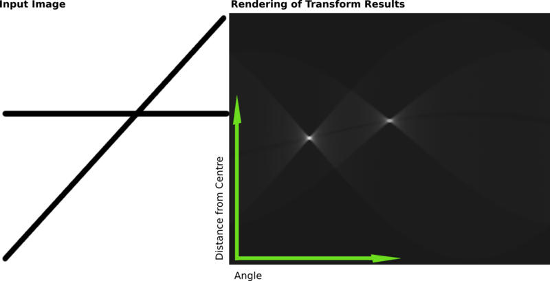
The results of this transform were stored in a matrix. Cell value represents the number of curves through any point. Higher cell values are rendered brighter. The two distinctly bright spots are the Hough parameters of the two lines. From these spots' positions, angle and distance from image center of the two lines in the input image can be determined.

[edit] Variations and extensions

[edit] Using the gradient direction to reduce the number of votes

An improvement suggested by O'Gorman and Clowes can be used to detect lines if one takes into account that the local gradient of the image intensity will necessarily be orthogonal to the edge. Since edge detection generally involves computing the intensity gradient magnitude, the gradient direction is often found as a side effect. If a given point of coordinates (x,y) happens to indeed be on a line, then the local direction of the gradient gives the θ parameter corresponding to said line, and the r parameter is then immediately obtained. (Shapiro and Stockman, 305) In fact, the real gradient direction is only estimated with a given amount of accuracy (approximately ±20°), which means that the sinusoid must be traced around the estimated angle, ±20°. This however reduces the computation time and has the interesting effect of reducing the number of useless votes, thus enhancing the visibility of the spikes corresponding to real lines in the image.

[edit] Kernel-based Hough transform

Fernandes and Oliveira ^[6] suggested an improved voting scheme for the Hough transform that allows a software implementation to achieve real-time performance even on relatively large images (e.g., 1280×960). The Kernel-based Hough transform uses the same (r,θ) parameterization proposed by Duda and Hart but operates on clusters of approximately collinear pixels. For each cluster, votes are cast using an oriented elliptical-Gaussian kernel that models the uncertainty associated with the best-fitting line with respect to the corresponding cluster. The approach not only significantly improves the performance of the voting scheme, but also produces a much cleaner accumulator and makes the transform more robust to the detection of spurious lines.

[edit] Hough transform of curves, and Generalised Hough transform

Although the version of the transform described above applies only to finding straight lines, a similar transform can be used for finding any shape which can be represented by a set of parameters. A circle, for instance, can be transformed into a set of three parameters, representing its center and radius, so that the Hough space becomes three dimensional. Arbitrary ellipses and curves can also be found this way, as can any shape easily expressed as a set of parameters. For more complicated shapes, the Generalised Hough transform is used, which allows a feature to vote for a particular position, orientation and/or scaling of the shape using a predefined look-up table.

[edit] Detection of 3D objects (Planes and cylinders)

Hough transform can also be used for the detection of 3D objects in range data or 3D point clouds. The extension of classical Hough transform for plane detection is quite straight forward. A plane is represented by its explicit equation z = a_x * x + a_y * y + d for which we can use a 3D Hough space corresponding to a_x, a_y and d. This extension suffers from the same problems as its 2D counter part i.e., near horizontal planes can be reliably detected, while the performance deteriorates as planar direction becomes vertical (big values of a_x and a_y amplify the noise in the data). This formulation of the plane has been used for the detection of planes in the point clouds acquired from airborne laser scanning ^[7] and works very well because in that domain all planes are nearly horizontal.

For generalized plane detection using Hough transform, the plane can be parametrized by its normal vector n (using spherical coordinates) and its distance from the origin ρ resulting in a three dimensional Hough space. This results in each point in the input data voting for a sinusoidal surface in the Hough space. The intersection of these sinusoidal surfaces indicates presence of a plane. ^[8]

Hough transform has also been used to find cylindrical objects in point clouds using a two step approach. The first step finds the orientation of the cylinder and the second step finds the position and radius. ^[9]

[edit] Using weighted features

One common variation detail. That is, finding the bins with the highest count in one stage can be used to constrain the range of values searched in the next.

[edit] Limitations

The Hough Transform is only efficient if a high number of votes fall in the right bin, so that the bin can be easily detected amid the background noise. This means that the bin must not be too small, or else some votes will fall in the neighboring bins, thus reducing the visibility of the main bin.^[10]

Also, when the number of parameters is large (that is, when we are using the Hough Transform with typically more than three parameters), the average number of votes cast in a single bin is very low, and those bins corresponding to a real figure in the image do not necessarily appear to have a much higher number of votes than their neighbors. Thus, the Hough Transform must be used with great care to detect anything other than lines or circles. This also, increases the complexity with each additional parameter. where A is the image space and m is the number of parameters. (Shapiro and Stockman, 310)

Finally, much of the efficiency of the Hough Transform is dependent on the quality of the input data: the edges must be detected well for the Hough Transform to be efficient. Use of the Hough Transform on noisy images is a very delicate matter and generally, a denoising stage must be used before. In the case where the image is corrupted by speckle, as is the case in radar images, the Radon transform is sometimes preferred to detect lines, since it has the nice effect of attenuating the noise through summation.

[edit] History

It was initially invented for machine analysis of bubble chamber photographs (Hough, 1959).

The Hough transform was patented as U.S. Patent 3,069,654 in 1962 and assigned to the U.S. Atomic Energy Commission with the name "Method and Means for Recognizing Complex Patterns". This patent uses a slope-intercept parametrization for straight lines, which awkwardly leads to an unbounded transform space since the slope can go to infinity.

The rho-theta parametrization universally used today was first described in

Duda, R. O. and P. E. Hart, "Use of the Hough Transformation to Detect Lines and Curves in Pictures," Comm. ACM, Vol. 15, pp. 11–15 (January, 1972),

although it was already standard for the Radon transform since at least the 1930s.

O'Gorman and Clowes' variation is described in

Frank O'Gorman, MB Clowes: Finding Picture Edges Through Collinearity of Feature Points. IEEE Trans. Computers 25(4): 449-456 (1976)