As a Data Scientist, I spend quite a bit of time thinking about Customer Lifetime Value (CLV) and how to model it. A strong CLV model is really a strong customer behavior model — the better you can predict next actions, the better you can quantify CLV.

作为数据科学家，我花了很多时间思考客户生命周期价值(CLV)以及如何对其建模。 强大的CLV模型实际上是强大的客户行为模型-您可以更好地预测下一步行动，就可以更好地量化CLV。

In this post, I hope to demonstrate, through both a toy and real-world example, why using aggregate statistics to judge the strength of a customer behavior model is a bad idea.

在本文中，我希望通过一个玩具实例和一个真实示例来说明为什么使用汇总统计数据来判断客户行为模型的优势是一个坏主意 。

Instead, the best CLV Model is the one that has the strongest predictions on the individual level. Data Scientists exploring Customer Lifetime Value should primarily, and perhaps only, use individual level metrics to fully understand the strengths and weaknesses of a CLV model.

相反，最好的CLV模型是在单个级别上具有最强预测的模型。 探索客户生命周期价值的数据科学家应主要(也许仅)使用个人级别的指标来全面了解CLV模型的优缺点。

第1章什么是CLV，为什么重要？ (Ch.1 What is CLV, and why is it important?)

While this is intended for Data Scientists, I wanted to address the business ramifications of this article, since understanding the business need will inform both why I hold certain opinions and why it is important for all of us to grasp the added benefit of a good CLV model.

虽然这是供数据科学家使用的，但我想解决本文的业务问题，因为了解业务需求将同时说明我为什么持有某些意见以及为什么对所有人来说，掌握良好CLV的额外好处很重要模型。

CLV: How much a customer will spend in the future

CLV ：客户将来会花费多少

CLV is a business KPI that has exploded in popularity over the past few years. The reason is obvious: if your company can accurately predict how much a customer will spend over the next couple months or years, you can tailor their experience to fit that budget. This has dramatic applications from marketing to customer service to overall business strategy.

CLV是一个业务KPI，在过去几年中Swift普及。 原因很明显：如果您的公司可以准确预测客户在未来几个月或几年内的支出，则可以根据预算调整他们的经验。 从营销到客户服务再到整体业务战略，这都有着引人注目的应用。

Here a quick list of business applications that accurate CLV can help empower:

以下是准确CLV可以帮助实现的业务应用程序的快速列表：

• Marketing Audience Generation营销受众生成
• Cohort Analysis队列分析
• Customer Service Ticket Ordering客户服务票务订购
• Marketing Lift Analysis营销提升分析
• CAC bid capping marketingCAC出价上限营销
• Discount Campaigns折扣活动
• VIP buying experiencesVIP购买体验
• Loyalty Programs会员计划
• Segmentation分割
• Board Reporting董事会报告

There’s plenty more, these are just the ones that come to my mind the fastest.

还有更多，这些只是我想到的最快的。

With so much business planning at stake, tech-savvy companies are busy scrambling to find which model can best capture CLV of their customer base. The most popular and commonly used customer lifetime value models benchmark their strength on aggregate metrics, using statistics like aggregate revenue percent error (ARPE). I know this because first hand many of my clients have compared their internal CLV models to mine using aggregate statistics.

面对如此多的业务计划，精通技术的公司正忙于寻找哪种模型最能抓住其客户群的CLV。 最流行和最常用的客户生命周期价值模型使用诸如总收入百分比误差(ARPE)之类的统计数据来衡量其在总指标上的优势。 我知道这一点是因为第一手资料我的许多客户已使用汇总统计数据将其内部CLV模型与我的模型进行比较。

I would argue that is a serious mistake.

我认为这是一个严重的错误。

The following 2 examples, one toy and one real, will hopefully demonstrate how aggregate statistics can both lead us astray and hide model shortcomings that are glaringly apparent at the individual level. This is especially prescient because most business use cases require a strong CLV model at the individual level, not just at the aggregate.

以下两个示例(一个玩具和一个真实玩具)将有望展示总体统计信息如何使我们误入歧途并掩盖模型缺陷，这些缺陷在个人层面上显而易见。 这是特别有先见之明的，因为大多数业务用例需要在单个级别(而不只是在总体级别)上使用强大的CLV模型。

第2章玩具示例 (Ch.2 A Toy Example)

When you rely on aggregate metrics and ignore the individual-level inaccuracies, you are missing a large part of the technical narrative. Consider the following example of 4 customers and their 1 year CLV:

当您依靠汇总指标并忽略个人级别的不准确性时，您会丢失很大一部分技术叙述。 考虑以下4个客户及其1年CLV的示例：

This example includes high, low, and medium CLV customers, as well as a churned customer, creating a nice distribution for a smart model to capture.

该示例包括高，低和中级CLV客户以及搅拌过的客户，从而为智能模型的捕获创建了良好的分布。

Now, consider the following validation metrics:

现在，请考虑以下验证指标：

1. MAE: Mean absolute error (The Average Difference between predictions)

   MAE ：平均绝对误差(预测之间的平均差)

3. ARPE: Aggregate revenue percent error (The overall difference between total revenue and predicted revenue)

3. ARPE ：总收入百分比误差(总收入与预期收入之间的总差)

MAE and is on the customer level, while ARPE and is an aggregate statistic. The lower the value for these validation metrics, the better.

MAE和处于客户级别，而ARPE和处于汇总统计。 这些验证指标的值越低越好。

This example will demonstrate how an aggregate statistic can bury the shortcomings of low-quality models.

此示例将演示汇总统计信息如何掩盖低质量模型的缺点。

To do so, compare a dummy guessing the mean to a CLV model off by 20% across the board.

为此，将假想平均数的假人与CLV模型进行比较，将其平均减少20％。

Model 1: The Dummy

模型1：假人

The dummy model will only guess $40 for every customer.

虚拟模型只会为每个客户猜测$ 40。

Model 2: CLV Model

模型2：CLV模型

This model tries to make an accurate model prediction at the customer level.

该模型试图在客户级别做出准确的模型预测。

We can use these numbers to calculate the three validation metrics.

我们可以使用这些数字来计算三个验证指标。

This example illustrates that a model that is considerably worse in the aggregate (the CLV model is worse by over 20%) is actually better at the individual level.

此示例说明，总体上较差的模型(CLV模型的差值超过20％)实际上在单个级别上更好。

To make this example even better, let’s add some noise to the predictions.

为了使这个示例更好，让我们在预测中添加一些噪点。

# Dummy Sampling:# randomly sampling a normal dist around $40 with a SD of $5np.random.normal (40,5,4)OUT: (44.88, 40.63, 40.35, 42.16)#CLV Sampling:# randomly sampling a normal dist around answer with a SD of $15max (0, np.random.normal (0,15)),max (0, np.random.normal (10, 15)),max (0, np.random.normal (50,15)),max  (0, np.random.normal (100, 15))OUT: (0, 17.48, 37.45, 81.41)

The results above indicate that even if an individual stat is a higher percentage than you would hope, the distribution of those CLV numbers is more in light with what we are looking for: a model that distinguishes high CLV customers from low CLV customers. If you only look at the aggregate metrics for a CLV model, you are missing a major part of the story, and you may end up choosing the wrong model for your business.

上面的结果表明，即使单个统计数据的百分比超出您的期望，这些CLV编号的分布也更加符合我们的需求：该模型将CLV高客户与低CLV客户区分开。 如果仅查看CLV模型的汇总指标，则可能会遗漏故事的大部分内容，最终可能会为您的业务选择错误的模型。

But even rolling up an error metric calculated at the individual level, such as MAE or alternatives like MAPE, can hide critical information about the strengths and weaknesses of your model. Mainly, its capacity to create an accurate distribution of CLV scores.

但是，即使汇总按单个级别计算的误差度量标准(例如MAE或MAPE等替代方案)，也可能隐藏有关模型优缺点的关键信息。 主要是其创建CLV分数的准确分布的能力。

To explore this further, let’s move to a more realistic example

为了进一步探讨这一点，让我们来看一个更现实的例子

第3章一个真实的例子 (Ch.3 A Real Example)

Congratulations! You, the Reader, have been hired as a Data Scientist by BottleRocket Brewing Co, an eCommerce company I just made up. (The data we will use is based on a real eCommerce company that I scrubbed for this post)

恭喜你！ 您(读者)已被我刚刚组建的电子商务公司BottleRocket Brewing Co聘为数据科学家。 (我们将使用的数据基于我为这篇文章整理的一家真正的电子商务公司)

Your first task as a Data Scientist: Choose the best CLV model for BottleRocket’s business…

作为数据科学家的首要任务：为BottleRocket的业务选择最佳的CLV模型…

…but what does “best” mean?

…但是“最佳”是什么意思？

Undeterred, you run an experiment with the following models:

不用担心，您可以使用以下模型进行实验：

1. Pareto/NBD Model (PNBD)

   帕累托/ NBD模型(PNBD)

The Pareto/NBD model is a very popular choice, and is the model under the hood of most data-driven CLV predictions today. To quote the documentation:

Pareto / NBD模型是一个非常受欢迎的选择，并且是当今大多数数据驱动的CLV预测的模型。 引用文档：

The Pareto/NBD model, introduced in 1987, combines the [Negative Binomial Distribution] for transactions of active customers with a heterogeneous dropout process, and to this date can still be considered a gold standard for buy-till-you-die models [Link]

1987年引入的Pareto / NBD模型将活跃客户交易的[负二项式分布]与异构退出过程结合在一起，到目前为止，仍可以认为是“买到卖-买-买”模型的黄金标准 [Link ]

But another way, the model learns two distributions, one for churn probability and the other for inter transaction-time (ITT) and makes CLV predictions by sampling from these distributions.

但是另一种方法是，该模型学习两种分布，一种用于流失概率，另一种用于交易间时间(ITT)，并通过从这些分布进行采样来进行CLV预测。

** Describing BTYD models in more technical detail is a bit out of scope of this article, which is focused on error metrics. Please drop a comment if you are interested in a more in-depth write-up about BTYD models and I’m happy to write a follow-on article!

**更详细地描述BTYD模型在本文的范围之内，本文的重点是错误度量。 如果您对BTYD模型的更深入的撰写感兴趣，请发表评论，我很乐意写一篇后续文章！

2. Gradient Boosted Machines (GBM)

2.梯度提升机(GBM)

Gradient Boosted Machines models are a popular machine learning model in which weak trees are trained and assembled together to make a strong overall classifier.

梯度提升机器模型是一种流行的机器学习模型，其中将弱树训练并组装在一起以构成一个强大的整体分类器。

** As with BTYD models, I won’t go into detail about how GBMs work but once again comment below if you’d like me to write up something on method/models

**与BTYD模型一样，我不会详细介绍GBM的工作原理，但是如果您希望我在方法/模型上写点东西，请在下面再次评论

3. Dummy CLV

3.虚拟CLV

This model is defined as simply:

该模型的定义很简单：

Calculate the average ITT for the businessCalculate the average spend over 1yrIf someone has not bought within 2x the average purchase time:    Predict $0Else:    Predict the average 1y spend

4. Very Dumb Dummy Model (Avg Dummy)

4.非常笨拙的虚拟模型(平均虚拟模型)

This model only guesses the average spend over 1yr for all customers. Included as a baseline for model performance

此模型仅猜测所有客户在1年以上的平均支出。 作为模型性能的基准

Ch.3.1 The Aggregate Metrics

第3.1章汇总指标

We can consolidate all of these models’ predictions into a nice little Pandas DataFrame `combined_result_pdf` that looks like:

我们可以将所有这些模型的预测合并为一个漂亮的小熊猫DataFrame`combined_result_pdf`，如下所示：

combined_result_pdf.head()

Given this customer table, we can calculate error metrics using the following code:

给定此客户表，我们可以使用以下代码来计算错误指标：

from sklearn.metrics import mean_absolute_erroractual = combined_result_pdf['actual']rev_actual = sum(actual)for col in combined_result_pdf.columns:    if col in ['customer_id', 'actual']:        continue    pred = combined_result_pdf[col]    mae = mean_absolute_error(y_true=actual, y_pred=pred)    print(col + ": ${:,.2f}".format(mae))

    rev_pred = sum(pred)    perc = 100*rev_pred/rev_actual    print(col + ": ${:,} total spend ({:.2f}%)".format(pred, perc))

With these four models, we tried to predict 1yr CLV for BottleRocket customers, ranked by MAE score:

对于这四种模型，我们尝试通过MAE得分对BottleRocket客户预测1年CLV：

Here are some interesting insights from this table:

下表列出了一些有趣的见解：

1. GBM appears to be the best model for CLVGBM似乎是CLV的最佳模型
2. PNBD, despite being a popular CLV, seems to be the worst. In fact, it’s worse than a simple if/else rule list, and only slightly better than a model only guesses the mean!尽管PNBD是受欢迎的CLV，但它似乎是最糟糕的。 实际上，它比简单的if / else规则列表还差，并且仅比模型仅猜测均值好一点！
3. Despite GBM being the best, it’s only a few dollars better than a dummy if/else rule list model尽管GBM是最好的，但仅比虚拟if / else规则列表模型好几美元

Point #3 especially has some interesting ramifications if the Data Scientist/Client accepts it. If the interpreter of these results actually believes that a simple if/else model can capture nearly all the complexity a GBM could capture, and better than the commonly used PNBD model, then obviously the “best” model would be the Dummy CLV once cost, speed of training, and interpretability are all factored in.

如果数据科学家/客户接受，第3点尤其会产生一些有趣的后果。 如果这些结果的解释者实际上认为，简单的if / else模型可以捕获GBM可以捕获的几乎所有复杂性，并且比常用的PNBD模型更好，那么显然，“最好的”模型是Dummy CLV，一旦投入使用，培训的速度和可解释性都是因素。

This brings us back to the original claim — that aggregate error metrics, even ones calculated on the individual level, hide some shortcomings of models. To demonstrate this, let’s rework our DataFrame into Confusion Matrices.

这使我们回到了最初的主张— 聚合错误度量标准，即使是在单个级别上计算出的误差度量标准，也隐藏了模型的某些缺点。 为了证明这一点，让我们将我们的DataFrame重做为混淆矩阵。

Mini Chapter: What is a Confusion Matrix?

迷你章节：什么是混淆矩阵？

From its name alone, understanding a confusion matrix sounds confusing & challenging. But it is crucial to understand the points being made in this post, as well as a powerful tool to add to your Data Science toolkit.

仅从其名称来看，理解混淆矩阵听起来就令人困惑和挑战。 但是，至关重要的是要了解本文中提出的要点以及将其添加到数据科学工具包中的强大工具。

A Confusion Matrix is a table that outlines the accuracy of classification, and what misclassifications are common by the model. A simple confusion matrix may look like this:

混淆矩阵是一个表格，概述了分类的准确性以及该模型常见的错误分类。 一个简单的混淆矩阵可能看起来像这样：

The diagonal on the above confusion matrix, highlighted Green, reflects correct predictions — predicting Cat when the it was actually a Cat etc. The rows will add up to 100%, allowing us to get a nice snapshot of how well our model captures Recall behavior, or the probability our model guesses correctly given a specific label.

上面混淆矩阵上的对角线(突出显示为绿色)反映了正确的预测-预测Cat实际上是Cat等时的行数。这些行的总和为100％，使我们可以很好地捕获模型捕获召回行为的方式，或我们的模型在给定特定标签的情况下正确猜测的可能性。

What we can also tell from the above confusion matrix is..

从上面的混淆矩阵中我们还可以看出。

1. The model is excellent at predicting Cat given the true label is Cat (Cat Recall is 90%)该模型非常适合预测Cat，因为真实标签为Cat(Cat召回率为90％)
2. The model has a difficult time distinguishing between Dogs and Cats, often misclassifying Dogs for Cats. This is the most common mistake made by the model.该模型很难区分狗和猫，经常将狗归为猫。 这是模型最常见的错误。
3. While it sometimes misclassifies a Cat as a Dog, it is far less common than other errors尽管有时会将猫误分类为狗，但它比其他错误少见

With this in mind, let’s explore how well our CLV models capture customer behavior using Confusion Matrices. A strong model would be able to correctly classify low value customers and high value customers as such. I prefer this method of visualization as opposed to something like a histogram of CLV scores because it reveals what elements of modelling the distribution are the strong and weak.

考虑到这一点，让我们探究我们的CLV模型如何使用混淆矩阵来捕获客户行为。 强大的模型将能够正确地将低价值客户和高价值客户分类。 我喜欢这种可视化方法，而不是像CLV得分的直方图那样，因为它揭示了建模分布的要素是强项还是弱项。

To achieve this, we will convert our monetary value predictions into quantiled CLV predictions of Low Medium High and Best. These will be drawn from the quantiles generated by each model’s predictions.

为了实现这一目标，我们将把货币价值预测转换为低中高和最佳的量化CLV预测。 这些将从每个模型的预测生成的分位数中得出。

The best model will correctly categorize customers into these 4 buckets of low/medium/high/best. Therefore each model we will make a confusion matrix of the following structure:

最佳模型将正确地将客户分类为这4个低/中/高/最佳桶。 因此，每个模型我们都将构成以下结构的混淆矩阵：

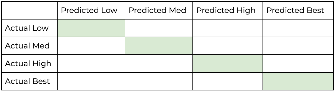
And the best model will have the most amount of predictions that fall within this diagonal.

最好的模型将在此对角线范围内具有最多的预测。

Ch. 3.2 The Individual Metrics

频道 3.2个人指标

These confusion matrices can be generated from our Pandas DF with the following code snippet:

这些混淆矩阵可以由我们的Pandas DF使用以下代码段生成：

from sklearn.metrics import confusion_matriximport matplotlib.patches as patchesimport matplotlib.colors as colors# Helper function to get quantilesdef get_quant_list(vals, quants):    actual_quants = []

    for val in vals:        if val > quants[2]:            actual_quants.append(4)        elif val > quants[1]:            actual_quants.append(3)        elif val > quants[0]:            actual_quants.append(2)        else:            actual_quants.append(1)    return(actual_quants)# Create Plotfig, axes = plt.subplots(nrows=int(num_plots/2)+(num_plots%2),ncols=2, figsize=(10,5*(num_plots/2)+1))fig.tight_layout(pad=6.0)tick_marks = np.arange(len(class_names))plt.setp(axes, xticks=tick_marks, xticklabels=class_names, yticks=tick_marks, yticklabels=class_names)# Pick colorscmap = plt.get_cmap('Greens')# Generate Quant Labelsplt_num = 0for col in combined_result_pdf.columns:    if col in ['customer_id', 'actual']:        continue    quants = combined_result_pdf[col]quantile(q=[0.25,0.5,0.75])    pred = combined_result_pdf[col]    pred_quants = get_quant_list(pred,quants)

    # Generate Conf Matrix    cm = confusion_matrix(y_true=actual_quants, y_pred=pred_quants)    ax = axes.flatten()[plt_num]    accuracy = np.trace(cm) / float(np.sum(cm))    misclass = 1 - accuracy     # Clean up CM code    cm = cm.astype('float') / cm.sum(axis=1)[:, np.newaxis] *100    ax.imshow(cm, interpolation='nearest', cmap=cmap)    ax.set_title('{} Bucketting'.format(col))    thresh = cm.max() / 1.5

    for i, j in itertools.product(range(cm.shape[0]), range(cm.shape[1])):        ax.text(j, i, "{:.0f}%".format(cm[i, j]), horizontalalignment="center", color="white" if cm[i, j] > thresh else "black")

    # Clean Up Chart    ax.set_ylabel('True label')    ax.set_xlabel('Predicted label')    ax.set_title('{}\naccuracy={:.0f}%'.format(col,100*accuracy))    ax.spines['top'].set_visible(False)    ax.spines['right'].set_visible(False)    ax.spines['bottom'].set_visible(False)    ax.spines['left'].set_visible(False)    for i in [-0.5,0.5,1.5,2.5]:        ax.add_patch(patches.Rectangle((i,i),        1,1,linewidth=2,edgecolor='k',facecolor='none'))    plt_num += 1

This produces the following Charts:

这将产生以下图表：

The coloring of the chart is how concentrated a certain prediction/actual classification is — the darker green, the more examples that fall within that square.

图表的颜色是某个预测/实际分类的集中程度-绿色越深，该正方形内的示例越多。

As with the example confusion matrix discussed above, the diagonal (highlighted with black lines) indicates appropriate classification of customers.

与上面讨论的示例混淆矩阵一样，对角线(用黑线突出显示)指示适当的客户分类。

Ch.3.3: Analysis

第3.3章：分析

Dummy Models (Top Row)

虚拟模型(顶行)

Dummy1, which is only predicting the average every time, has a distribution of ONLY the mean. It makes no distinction between high or low value customers.

Dummy1每次仅预测平均值，其分布只有平均值。 高价值客户与低价值客户没有区别。

Only slightly better, Dummy2 predicts either $0 or the average. This means it can make some claim about distribution, and in fact, capture 81% and 98% of the lowest and highest value customers respectively.

Dummy2只能预测好一点，即$ 0或平均值。 这意味着它可以对分销有所要求，实际上，它们分别吸引了81％和98％的最低和最高价值客户。

But the major issue with these models, which was not apparent when looking at MAE (but obvious if you know how their labels were generated), is that these models have very little sophistication when it comes to distinguishing between customer segments. For all of our business applications listed in Ch.1, which is the entire point of building a strong CLV model, distinguishing between customer types is essential to success

但是，这些模型的主要问题在看MAE时并不明显(如果您知道它们的标签是如何生成的，则很明显)，当区分客户群时，这些模型的复杂性很小。 对于第1章中列出的所有业务应用程序(这是构建强大的CLV模型的全部要点)，区分客户类型对于成功至关重要

CLV Models (Bottom Row)

CLV模型(底行)

First, don’t let the overall accuracy scare you. In the same way that we can hide the truth through aggregate statistics, we can hide the strength of distribution modelling through a rolled-out accuracy metric.

首先，不要让整体准确性吓到您。 就像我们可以通过聚合统计信息隐藏真相一样，我们可以通过推出的准确性度量标准来隐藏分布建模的强度。

Second, it is pretty clear from this visual, as opposed to the previous table, that there is a reason the dummy models are named as such — these second row models are actually capturing a distribution. Even with Dummy2 capturing a much higher percentage of low value customers — this can just be an artifact of having a long-tail CLV distribution. Clearly, these are the models you want to be choosing between.

其次，与上一张表相比，从视觉上可以很明显地看出，有一个假模型被如此命名的原因-这些第二行模型实际上是在捕获分布。 即使Dummy2捕获了更高比例的低价值客户，这也可能只是具有长尾CLV分配的产物。 显然，这些是您要在其中选择的模型。

Looking at the diagonal, we can see that GBM has major improvements in predicting most categories across the board. Major mislabellings — missing by two squares — is down considerably. The biggest increase on the GBM side is on recognizing medium level customers, which is a nice sign that the distribution is healthy and our predictions are realistic.

纵观对角线，我们可以看到GBM在全面预测大多数类别方面有重大改进。 主要的错误标签-减少了两个正方形-大大减少了。 GBM方面的最大增长是对中级客户的认可，这很好地表明了分布状况良好且我们的预测是现实的。

第4章 结束 (Ch4. The End)

If you just skimmed this article, you may want to conclude that GBM is a better CLV model. And that may be true, but model selection is more complicated. Some questions you would want to ask:

如果您只是浏览了这篇文章，则可能要得出结论，GBM是更好的CLV模型。 可能是这样，但是模型选择更加复杂。 您想问的一些问题：

• Do I want to predict many years into the future?我想预测未来很多年吗？
• Do I want to predict churn?我要预测客户流失吗？
• Do I want to predict the number of transactions?我要预测交易数量吗？
• Do I have enough data to run a supervised model?我是否有足够的数据来运行监督模型？
• Do I care about explainability?我是否在乎可解释性？

Are of these questions, while not related to the thesis of this article, would need to be answered before you swap out your model for a GBM.

这些问题是否与本文的主题无关，但在将模型换成GBM之前需要先回答。

First underlying variable to consider when choosing the model is the company’s data you are working with. Often BTYD models work well, and are comparable to ML alternatives. But BTYD models make some strong assumptions about customer behavior, so if these assumptions are broken, they perform sub-optimally. Running a model comparison is crucial to making the right model decision.

选择模型时要考虑的第一个基础变量是您正在使用的公司数据。 通常BTYD模型可以很好地工作，并且可以与ML替代品相媲美。 但是BTYD模型对客户行为做出了一些强有力的假设，因此，如果这些假设被破坏，它们的表现将不尽人意。 运行模型比较对于做出正确的模型决策至关重要。

While the issues at the individual level are apparent for the dummy models, often companies will fall prey to these issues by running a “naive”/”simple”/”excel-based” model to do this exact thing — attempt to apply an aggregate number across your entire customer base. At some companies, CLV can be as simply defined by dividing revenue equally among all customers. This may work for a board report or two, but in reality, this is not an adequate way to calculate such a complex number. Truth is, not all customers are created equal, and the sooner your company shifts their attention away from aggregate customer metrics to strong individual-level predictions, the more effectively you can market, strategize and ultimately find your best customers.

尽管对于虚拟模型而言，个人层面的问题是显而易见的，但公司通常会通过运行“幼稚” /“简单” /“基于excel的”模型来做这些确切的事情，从而成为这些问题的猎物-尝试应用汇总您整个客户群中的数量。 在某些公司中，CLV可以简单地定义为将收入平均分配给所有客户。 这可能适用于一两个董事会的报告，但实际上，这并不是计算如此复杂数字的适当方法。 事实是，并非所有客户都是平等创造的，并且您的公司越早将其注意力从总客户指标转移到强有力的个人水平预测上，您就可以越有效地进行市场营销，制定战略并最终找到最佳客户。

Hope this was as enjoyable and informative to read about as it was to write about.

希望阅读和撰写这篇文章一样愉快和有益。

Thanks for reading!

谢谢阅读！