线性回归非线性回归_了解线性回归
线性回归非线性回归
Let’s say you’re looking to buy a new PC from an online store (and you’re most interested in how much RAM it has) and you see on their first page some PCs with 4GB at $100, then some with 16 GB at $1000. Your budget is $500. So, you estimate in your head that given the prices you saw so far, a PC with 8 GB RAM should be around $400. This will fit your budget and decide to buy one such PC with 8 GB RAM.
假设您要从网上商店购买一台新PC(并且您最感兴趣的是它有多少RAM),并且在他们的首页上看到一些4GB价格为100美元的PC,然后一些16GB价格为1000美元的PC 。 您的预算是$ 500。 因此,您估计自己的价格,考虑到到目前为止的价格,一台具有8 GB RAM的PC应该约为400美元。 这将适合您的预算,并决定购买一台具有8 GB RAM的PC。
This kind of estimations can happen almost automatically in your head without knowing it’s called linear regression and without explicitly computing a regression equation in your head (in our case: y = 75x - 200).
这种估算几乎可以在您的头脑中自动发生,而无需知道这是线性回归,也无需在您的头脑中显式计算回归方程(在我们的情况下:y = 75x-200)。
So, what is linear regression?
那么,什么是线性回归?
I will attempt to answer this question simply:
我将尝试简单地回答这个问题:
Linear regression is just the process of estimating an unknown quantity based on some known ones (this is the regression part) with the condition that the unknown quantity can be obtained from the known ones by using only 2 operations: scalar multiplication and addition (this is the linear part). We multiply each known quantity by some number, and then we add all those terms to obtain an estimate of the unknown one.
线性回归只是基于一些已知量(这是回归部分)估算未知量的过程,条件是只能使用以下两个操作从已知量中获取未知量:标量乘法和加法(这是线性部分)。 我们将每个已知数量乘以某个数字,然后将所有这些项相加以获得未知数量的估计值。
It may seem a little complicated when it is described in its formal mathematical way or code, but, in fact, the simple process of estimation as described above you probably already knew way before even hearing about machine learning. Just that you didn’t know that it is called linear regression.
以正式的数学方式或代码描述它似乎有些复杂,但是,实际上,如上所述的简单估算过程,您甚至在听说机器学习之前就已经知道了。 只是您不知道它称为线性回归。
Now, let’s dive into the math behind linear regression.
现在,让我们深入了解线性回归背后的数学原理。
In linear regression, we obtain an estimate of the unknown variable (denoted by y; the output of our model) by computing a weighted sum of our known variables (denoted by xᵢ; the inputs) to which we add a bias term.
在线性回归中,我们通过计算已知变量(以xᵢ表示;输入)的加权和来获得未知变量(以y表示;模型的输出)的估计值,并在该变量上加上偏差项。
Where n is the number of data points we have.
其中n是我们拥有的数据点数。
Adding a bias is the same thing as imagining we have an extra input variable that’s always 1 and using only the weights. We will consider this case to make the math notation a little easier.
添加一个偏差与想象我们有一个总是为1且仅使用权重的额外输入变量相同。 我们将考虑这种情况,以使数学符号更容易些。
Where x₀ is always 1, and w₀ is our previous b.
其中X 0始终为1,W 0和是我们以前湾
To make the notation a little easier, we will transition from the above sum notation to matrix notation. The weighted sum in the equation above is equivalent to the multiplication of a row-vector of all the input variables with a column-vector of all the weights. That is:
为了使表示法更容易一点,我们将从上面的总和表示法转换为矩阵表示法。 上式中的加权和等于所有输入变量的行向量与所有权重的列向量相乘。 那是:

The equation above is for just one data point. If we want to compute the outputs of more data points at once, we can concatenate the input rows into one matrix which we will denote by X. The weights vector will remain the same for all those different input rows and we will denote it by w. Now y will be used to denote a column-vector with all the outputs instead of just a single value. This new equation, the matrix form, is given below:
上面的等式仅适用于一个数据点。 如果要一次计算更多数据点的输出,可以将输入行连接到一个矩阵中,用X表示。 对于所有这些不同的输入行,权重向量将保持相同,我们将用w表示它。 现在, y将用于表示具有所有输出的列向量,而不仅仅是单个值。 这个新的方程,矩阵形式,如下:
Given an input matrix X and a weights vector w, we can easily get a value for y using the formula above. The input values are assumed to be known, or at least to be easy to obtain.
给定一个输入矩阵X和一个权重向量w ,我们可以使用上面的公式轻松得出y的值。 假定输入值是已知的,或者至少易于获得。
But the problem is: How do we obtain the weights vector?
但是问题是:我们如何获得权重向量?
We will learn them from examples. To learn the weights, we need a dataset in which we know both x and y values, and based on those we will find the weights vector.
我们将从示例中学习它们。 要学习权重,我们需要一个既知道x值又知道y值的数据集,然后根据这些数据集找到权重向量。
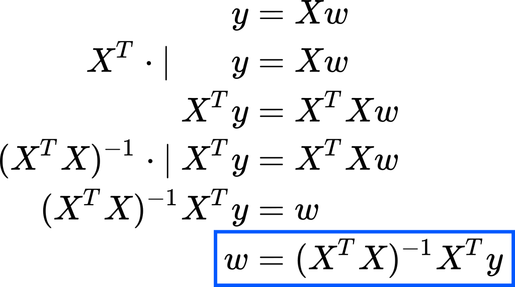
If our data points are the minimum required to define our regression line (one more than the number of inputs), then we can simply solve equation (1) for w:
如果我们的数据点是定义回归线所需的最小值(比输入数多一个),那么我们可以简单地为w求解方程式(1):

We call this thing a regression line, but actually, it is a line only for 1 input. For 2 inputs it will be a plane, for 3 inputs it will be some kind of “3D plane”, and so on.
我们称此为回归线,但实际上,这是仅用于1个输入的线。 对于2个输入,它将是一个平面,对于3个输入,它将是某种“ 3D平面”,依此类推。
Most of the time the requirement for the solution above will not hold. Most of the time, our data points will not perfectly fit a line. There will be some random noise around our regression line, and we will not be able to obtain an exact solution for w. However, we will try to obtain the best possible solution for w so that the error is minimal.
在大多数情况下,上述解决方案的要求将不成立。 在大多数情况下,我们的数据点不会完全符合一条线。 我们的回归线附近会有一些随机噪声,因此我们将无法获得w的精确解。 但是,我们将尝试获得w 的最佳解决方案 ,以使误差最小。
If equation (1) doesn’t have a solution, this means that y doesn’t belong to the column space of X. So, instead of y, we will use the projection of y onto the column space of X. This is the closest vector to y that also belongs to the column space of X. If we multiply (on the left) both sides of eq. (1) by the transpose of X, we will get an equation in which this projection is considered. You can find out more about the linear algebra approach of solving this problem in this lecture by Gilbert Strang from MIT.
如果等式(1)没有解,则意味着y不属于X的列空间。 因此,我们将使用y到X的列空间上的投影代替y 。 这是最接近y的向量,它也属于X的列空间。 如果我们(在左边)乘以等式的两边。 (1)通过X的转置,我们将得到一个考虑该投影的方程。 您可以在MIT的Gilbert Strang的讲座中找到有关解决此问题的线性代数方法的更多信息。
Although this solution requires fewer restrictions on X than our previous one, there are some cases in which it still doesn’t work; we will see more about this issue below.
尽管此解决方案对X的限制比我们以前的解决方案要少,但是在某些情况下它仍然不起作用。 我们将在下面看到有关此问题的更多信息。
Another way to get a solution for w is by using calculus. The main idea is to define an error function, then use calculus to find the weights that minimize this error function.
获得w解决方案的另一种方法是使用微积分。 主要思想是定义一个误差函数,然后使用微积分找到使该误差函数最小的权重。
We will define a function f that takes as input a weights vector and gives us the squared error these weights will generate on our linear regression problem. This function simply looks at the difference between each true y from our dataset and the estimated y of the regression model. Then squares all these differences and adds them up. In matrix notation, this function can be written as:
我们将定义一个函数f ,该函数将权重向量作为输入,并给出这些权重将在线性回归问题上产生的平方误差。 此函数只是查看数据集中每个真实y与回归模型的估计y之间的差异。 然后将所有这些差异平方并加总。 用矩阵表示法,该函数可以写为:
If this function has a minimum, it should be at one of the critical points (the points where the gradient ∇f is 0). So, let’s find the critical points. If you’re not familiar with matrix differentiation, you can have a look at this Wikipedia article.
如果此函数具有最小值,则应位于临界点之一(梯度∇f为0的点)上。 因此,让我们找到关键点。 如果您不熟悉矩阵微分,可以看看这篇 Wikipedia文章。
We start by computing the gradient:
我们首先计算梯度:

Then we set it equal to 0, and solve for w:
然后将其设置为0,并求解w :

We got one critical point. Now we should figure out if it is a minimum or maximum point. To do so, we will compute the Hessian matrix and establish the convexity/concavity of the function f.
我们有一个关键点。 现在我们应该确定它是最小还是最大点。 为此,我们将计算Hessian矩阵并建立函数f的凸/凹度。
Now, what can we observe about H? If we take any real-valued vector z and multiply it on both sides of H, we will get:
现在,我们可以观察到关于H的什么? 如果我们取任何实值向量z并将其在H的两边相乘,我们将得到:
Because f is a convex function, this means that our above-found solution for w is a minimum point and that’s exactly what we were looking for.
因为f是一个凸函数,所以这意味着我们上面找到的w的解决方案是一个最小点,而这正是我们想要的。
As you probably noticed, we got the same solution for w by using both the previous linear algebra approach and this calculus way of finding the weights. We can think of it as either the solution of the matrix equation when we replace y by the projection of y onto the column space of X or the point that minimizes the sum of squared errors.
您可能已经注意到,通过使用以前的线性代数方法和这种求权的演算方法,我们得到了与w相同的解决方案。 我们可以将其视为矩阵方程的解,当我们将y替换为y在X的列空间上的投影或最小化平方误差之和的点时。
Does this solution always work? No.
此解决方案是否始终有效? 没有。
It is less restrictive than the trivial solution: w = X⁻¹ y in which we need X to be a square non-singular matrix, but it still needs some conditions to hold. We need Xᵀ X to be invertible, and for that X needs to have full column rank; that is, all its columns to be linearly independent. This condition is typically met if we have more rows than columns. But if we have fewer data examples than input variables, this condition cannot be true.
它比一般解的约束要小: w = X y ,其中我们需要X为正方形非奇异矩阵,但仍然需要一些条件来保持。 我们需要XᵀX是可逆的,并且为此X 需要具有完整的列秩 ; 也就是说,其所有列都是线性独立的。 如果我们的行多于列,通常会满足此条件。 但是,如果我们的数据示例少于输入变量,则此条件不能成立。
This requirement that X has full column rank is closely related to the convexity of f. If you look above at the little proof that f is convex, you can notice that, if X has full column rank, then X z cannot be the zero vector (assuming z ≠ 0), and this implies that H is positive definite, hence f is strictly convex. If f is strictly convex it can have only one minimum point, and this explains why this is the case in which we can have a closed-form solution.
X具有完整列等级的要求与f的凸性密切相关。 如果您在上面看f是凸的小证明,您会注意到,如果X具有完整的列秩,则X z不能为零向量(假设z≠0 ),这意味着H是正定的,因此f 严格是凸的。 如果f是严格凸的,则它只能有一个最小点,这解释了为什么我们可以有一个封闭形式的解。
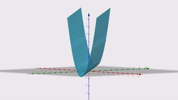
On the other hand, if X doesn’t have full column rank, then there will be some z ≠ 0 for which X z = 0, and therefore f is non-strictly convex. This means that f may not have a single minimum point, but a valley of minimum points which are equally good, and our closed-form solution is not able to capture all of them. Visually, the case of a not full column rank X looks something like this in 3D:
另一方面,如果X没有完整的列级,则将存在z≠0且 X z = 0 ,因此f是非严格凸的。 这意味着f可能没有一个最小点,但是一个最小点的谷值同样好,并且我们的封闭式解决方案无法捕获所有这些点。 从视觉上看,列级别X不完整的情况在3D中看起来像这样:
A method that will give us a solution even in this scenario is Stochastic Gradient Descent (SGD). This is an iterative method that starts at a random point on the surface of the error function f, and then, at each iteration, it goes in the negative direction of the gradient ∇f towards the bottom of the valley.
即使在这种情况下,也可以为我们提供解决方案的一种方法是随机梯度下降 (SGD)。 这是一种迭代方法,从误差函数f的表面上的随机点开始,然后在每次迭代时,它沿梯度∇f的负方向向谷底移动。
This method will always give us a result (even if sometimes it requires a large number of iterations to get to the bottom); it doesn’t need any condition on X.
这种方法将始终为我们提供结果(即使有时它需要进行大量迭代才能达到最低要求); 它在X上不需要任何条件。
Also, to be more efficient computationally, it doesn’t use all the data at once. Our data matrix X is split vertically into batches. At each iteration, an update is done based only on one such batch.
另外,为了提高计算效率,它不会一次使用所有数据。 我们的数据矩阵X垂直分为几批。 在每次迭代中,仅基于一个这样的批次进行更新。
In the case of not full column rank X, the solution will not be unique; among all those points in the “minimum valley”, SGD will give us only one that depends on the random initialization and the randomization of the batches.
如果列级别X不完整,则解决方案将不是唯一的; 在“最小谷”中的所有这些点中,SGD将只给我们一个依赖于批次的随机初始化和随机化的点。
SGD is a more general method that is not tied only to linear regression; it is also used in more complex machine learning algorithms like neural networks. But an advantage that we have here, in the case of least-squares linear regression, is that, due to the convexity of the error function, SGD cannot get stuck into local minima, which is often the case in neural networks. When this method will reach a minimum, it will be a global one. Below is a brief sketch of this algorithm:
SGD是一种更通用的方法,不仅限于线性回归; 它也用于更复杂的机器学习算法(如神经网络)中。 但是在最小二乘线性回归的情况下,我们在这里拥有的一个优势是,由于误差函数的凸性,SGD不会陷入局部最小值,这在神经网络中通常是这样。 当此方法达到最小值时,它将是全局方法。 下面是该算法的简要示意图:

Where α is a constant called learning rate.
其中α是一个常数,称为学习率 。
Now, if we plug in the gradient as computed above in this article, we get the following which is specifically for least-squares linear regression:
现在,如果我们按照本文上面的计算方法插入渐变,则会得到以下内容,这些内容专门用于最小二乘线性回归:
And that’s it for now. In the next couple of articles, I will also show how to implement linear regression using some numerical libraries like NumPy, TensorFlow, and PyTorch.
仅此而已。 在接下来的几篇文章中,我还将展示如何使用一些数字库(如NumPy,TensorFlow和PyTorch)实现线性回归。
I hope you found this information useful and thanks for reading!
我希望您发现此信息有用,并感谢您的阅读!
翻译自: https://towardsdatascience.com/understanding-linear-regression-eaaaed2d983e
线性回归非线性回归
http://www.taodudu.cc/news/show-995265.html
相关文章:
- 数据图表可视化_数据可视化如何选择正确的图表第1部分
- 使用python和javascript进行数据可视化
- github gists 101使代码共享漂亮
- 大熊猫卸妆后_您不应错过的6大熊猫行动
- jdk重启后步行_向后介绍步行以一种新颖的方式来预测未来
- scrapy模拟模拟点击_模拟大流行
- plsql中导入csvs_在命令行中使用sql分析csvs
- 交替最小二乘矩阵分解_使用交替最小二乘矩阵分解与pyspark建立推荐系统
- 火种 ctf_分析我的火种数据
- 分析citibike数据eda
- 带有postgres和jupyter笔记本的Titanic数据集
- 机器学习模型 非线性模型_机器学习模型说明
- 算命数据_未来的数据科学家或算命精神向导
- 熊猫数据集_熊猫迈向数据科学的第三部分
- 充分利用UC berkeleys数据科学专业
- 铁拳nat映射_铁拳如何重塑我的数据可视化设计流程
- 有效沟通的技能有哪些_如何有效地展示您的数据科学或软件工程技能
- vue取数据第一个数据_我作为数据科学家的第一个月
- rcp rapido_为什么气流非常适合Rapido
- 算法组合 优化算法_算法交易简化了风险价值和投资组合优化
- covid 19如何重塑美国科技公司的工作文化
- 蒙特卡洛模拟预测股票_使用蒙特卡洛模拟来预测极端天气事件
- 微生物 研究_微生物监测如何工作,为何如此重要
- web数据交互_通过体育运动使用定制的交互式Web应用程序数据科学探索任何数据...
- 熊猫数据集_用熊猫掌握数据聚合
- 数据创造价值_展示数据并创造价值
- 北方工业大学gpa计算_北方大学联盟仓库的探索性分析
- missforest_missforest最佳丢失数据插补算法
- 数据可视化工具_数据可视化
- 使用python和pandas进行同类群组分析
线性回归非线性回归_了解线性回归相关推荐
- 线性回归 非线性回归_线性回归的解释
线性回归 非线性回归 Linear Regression is the most talked-about term for those who are working on ML and stati ...
- 线性回归 假设_违反线性回归假设的后果
线性回归 假设 动机 (Motivation) Recently, a friend learning linear regression asked me what happens when ass ...
- python多元非线性回归_利用Python进行数据分析之多元线性回归案例
线性回归模型属于经典的统计学模型,该模型的应用场景是根据已知的变量(自变量)来预测某个连续的数值变量(因变量).例如,餐厅根据每天的营业数据(包括菜谱价格.就餐人数.预定人数.特价菜折扣等)预测就餐规 ...
- 机器学习 线性回归算法_探索机器学习算法简单线性回归
机器学习 线性回归算法 As we dive into the world of Machine Learning and Data Science, one of the easiest and f ...
- python多元线性回归实例_利用Python进行数据分析之多元线性回归案例
线性回归模型属于经典的统计学模型,该模型的应用场景是根据已知的变量(自变量)来预测某个连续的数值变量(因变量).例如,餐厅根据每天的营业数据(包括菜谱价格.就餐人数.预定人数.特价菜折扣等)预测就餐规 ...
- 回归分析之线性回归(N元线性回归)
标签(空格分隔): 回归分析 二元线性回归 多元线性回归 打开微信扫一扫,关注微信公众号[数据与算法联盟] 转载请注明出处:http://blog.csdn.net/gamer_gyt 博主微博:ht ...
- R语言使用lm函数构建简单线性回归模型(建立线性回归模型)、拟合回归直线、使用attributes函数查看线性回归模型的属性信息、获取模型拟合对应的残差值residuals
R语言使用lm函数构建简单线性回归模型(建立线性回归模型).拟合回归直线.使用attributes函数查看线性回归模型的属性信息.获取模型拟合对应的残差值residuals 目录
- R语言使用lm函数构建简单线性回归模型(建立线性回归模型)、拟合回归直线、可视化散点图并添加简单线性回归直线、添加模型拟合值数据点、添加拟合值点和实际数据点之间的线段表示残差大小、col参数自定义设置
R语言使用lm函数构建简单线性回归模型(建立线性回归模型).拟合回归直线.可视化散点图并添加简单线性回归直线.添加模型拟合值数据点.添加拟合
- R语言使用lm函数构建简单线性回归模型(建立线性回归模型)、拟合回归直线、使用residuls函数从模型中提取每个样本点的残差值、可视化残差与拟合值之间的散点图来看残差的分布模式
R语言使用lm函数构建简单线性回归模型(建立线性回归模型).拟合回归直线.使用residuls函数从模型中提取每个样本点的残差值.可视化残差与拟合值之间的散点图来看残差的分布模式 目录
最新文章
- 一款高颜值的MySQL管理工具:Sequel Pro
- n分频器 verilog_基于Verilog的分频器实现
- javafx响应式布局_JavaFX的响应式设计
- idea设置中文界面_《英雄联盟手游》设置界面中文翻译图分享 外服汉化界面一览...
- pixel 6 root
- Smokeping的参数使用说明
- python 迭代器协议斐波那契数列
- 我必须得告诉大家的 MySQL 优化原理
- (转)给趋势投资信仰充值:动量模型百年赚钱史
- 华为工程师都没有解决的问题,华为交换机acl不能使用易维版显示
- python爬虫爬取网站视频_python3爬虫爬取视频(一)
- 安卓逆向学习 之 KGB Messenger的writeup(2)
- magento 开发 -- 入门深入理解第五章 – Magento资源配置
- 回溯法采用的搜索策略_下列那种函数是回溯法中为避免无效搜索采取的策略( )_学小易找答案...
- html鼠标悬停显示内容
- 关于我在刷题时用OJ判题发现的cout相较于printf严重超时的问题
- matlab做TSP,MATLAB TSP问题
- DayDreamer's Blog Qt资料整理~待续
- FPAG—计数器—BCD译码器—Verilog
- 卫星导航定位技术二:由星历参数求解卫星时空位置