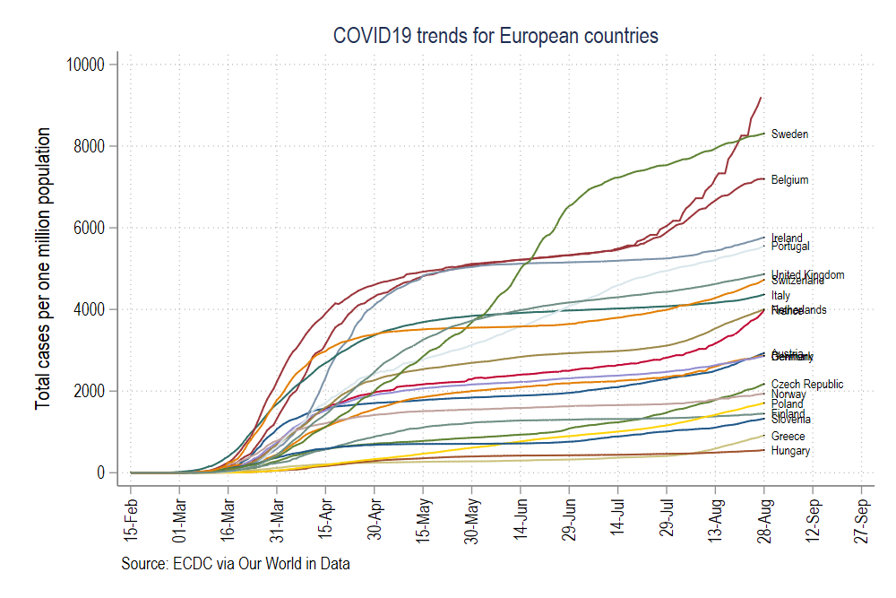
This guide will cover an important, yet, under-explored part of Stata: the use of custom color schemes. In summary, we will learn how to go from this graph:

本指南将涵盖Stata的一个重要但尚未充分研究的部分：自定义配色方案的使用。 总而言之，我们将学习如何从该图开始：

to this graph which implements a matplotlib color scheme, typically used in R and Python graphs, in Stata:

该图实现了matplotlib配色方案 ，通常在Stata中用于R和Python图：

This guide also touches upon advanced use of locals and loops which are essential for automation of tasks in Stata. Therefore, the guide assumes a basic knowledge of Stata commands. Understanding the underlying underlying logic here can also be applied to various Stata routines beyond generating graphs.

本指南还涉及高级使用局部变量和循环，这对于Stata中的任务自动化至关重要。 因此，本指南假定您具有Stata命令的基本知识。 除了生成图形外，了解此处的基本逻辑还可以应用于各种Stata例程。

This guide build on the first article where data management, folder structures, and an introduction to automation of tasks are discussed in detail. While it is highly recommended to follow the first guide to set up the data and the folders, for the sake of completeness, some basic information is repeated here.

本指南以第一篇文章为基础 ，其中详细讨论了数据管理，文件夹结构以及任务自动化的简介。 虽然强烈建议您遵循第一本指南来设置数据和文件夹，但是为了完整起见，此处重复一些基本信息。

The guide follows a specific folder structure, in order to track changes in files. This folder structure and code used in the first guide can be downloaded from Github.

该指南遵循特定的文件夹结构，以便跟踪文件中的更改。 可以从Github下载此第一指南中使用的文件夹结构和代码。

In case you are starting from scratch, create a main folder and the following five sub-folders within the root folder:

如果您是从头开始，请在根文件夹中创建一个主文件夹和以下五个子文件夹：

This will allow you to use the code, that makes use of relative paths, given in this guide.

这将允许您使用本指南中提供的使用相对路径的代码。

The guide is split into five steps:

该指南分为五个步骤：

• Step 1: provides a quick summary on setting up the COVID-19 dataset from Our World in Data.

  第1步 ：提供有关从Our World in Data中建立COVID-19数据集的快速摘要。

• Step 2: discusses custom graph schemes for cleaning up the layout

  步骤2 ：讨论用于清理布局的自定义图形方案

• Step 3: introduces line graphs and their various elements

  步骤3 ：介绍折线图及其各种元素

• Step 4: introduces color palettes and how to integrate them into line graphs

  第4步 ：介绍调色板以及如何将它们集成到折线图中

• Step 5: shows how the whole process of generating graphs with custom color schemes can be automated using loops and locals

  步骤5 ：展示如何使用循环和局部变量自动生成带有自定义配色方案的图形的整个过程

步骤1：重新整理资料 (Step 1: A refresher on the data)

In case you are starting from scratch, start a new dofile, and set up the data using the following commands:

如果您是从头开始的，请启动一个新的文件，然后使用以下命令设置数据：

clearcd <your main directory here with sub-folders shown above>*************************************** our worldindata ECDC dataset***********************************insheet using "https://covid.ourworldindata.org/data/ecdc/full_data.csv", clearsave ./raw/full_data_raw.dta, replacegen year  = substr(date,1,4)gen month = substr(date,6,2)gen day   = substr(date,9,2)destring year month day, replacedrop dategen date = mdy(month,day,year)format date %tdDD-Mon-yyyydrop year month daygen date2 = dateorder date date2drop if date2 < 21915gen group = .replace group = 1 if /// location == "Austria"         | ///  location == "Belgium"         | /// location == "Czech Republic"  | /// location == "Denmark"         | /// location == "Finland"         | /// location == "France"          | /// location == "Germany"         | /// location == "Greece"          | /// location == "Hungary"         | /// location == "Italy"           | /// location == "Ireland"         | /// location == "Netherlands"     | /// location == "Norway"          | /// location == "Poland"          | /// location == "Portugal"        | /// location == "Slovenia"        | /// location == "Slovak Republic" | /// location == "Spain"           | /// location == "Sweden"          | /// location == "Switzerland"     | /// location == "United Kingdom"keep if group==1ren location countrytab countrycompresssave "./temp/OWID_data.dta", replace**** adding the population datainsheet using "https://covid.ourworldindata.org/data/ecdc/locations.csv", cleardrop countriesandterritories population_yearren location countrycompresssave "./temp/OWID_pop.dta", replace**** merging the two datasetsuse ./temp/OWID_data, clearmerge m:1 country using ./temp/OWID_popdrop if _m!=3drop _m***** generating population normalized variablesgen total_cases_pop  = (total_cases  / population) * 1000000gen total_deaths_pop = (total_deaths / population) * 1000000***** clean up the datedrop if date < 21960format date %tdDD-Monsumm date***** identify the last datesumm dategen tick = 1 if date == `r(max)'***** save the filecompresssave ./master/COVID_data.dta, replace

步骤2：自定义图形方案 (Step 2: Custom graph schemes)

In the first guide, we learnt how to make line graphs using the Stata’s xtline command. This was done by declaring the data to be a panel dataset. To summarize, we use the following commands to generate a panel data line graph:

在第一个指南中 ，我们学习了如何使用Stata的xtline命令制作线图。 这是通过将数据声明为面板数据集来完成的。 总而言之，我们使用以下命令来生成面板数据折线图：

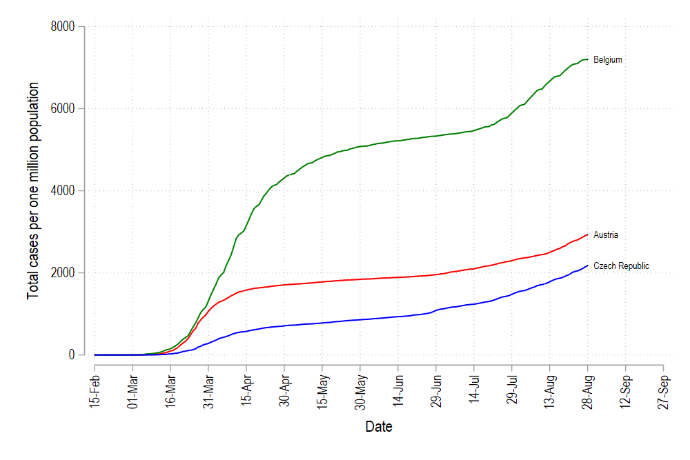
summ datelocal start = `r(min)'local end   = `r(max)' + 30xtline total_cases_pop /// , overlay ///  addplot((scatter total_cases_pop date if tick==1, mcolor(black) msymbol(point) mlabel(country) mlabsize(vsmall) mlabcolor(black))) ///  ttitle("") ///  tlabel(`start'(15)`end', labsize(small) angle(vertical) grid) ///  title(COVID19 trends for European countries) ///  note(Source: ECDC via Our World in Data) ///  legend(off) ///  graphregion(fcolor(white)) ///  scheme(s2color)graph export ./graphs/medium2_graph1.png, replace wid(1000)

which gives us this figure:

这给了我们这个数字：

This figure uses the default color s2 color scheme in Stata where we manually adjusted the background colors, axes, labels, and headings. The font is set to Arial Narrow. In the code above, we add an additional feature to the graph code, scheme(s2color) to manually define which scheme we want to use.

此图使用Stata中的默认颜色s2配色方案，在该方案中我们手动调整了背景色，轴，标签和标题。 字体设置为Arial Narrow。 在上面的代码中，我们在图形代码中添加了一个额外的功能Scheme(s2color)，以手动定义我们要使用的方案。

Rather than customizing minor elements of graphs ourselves, we can also rely on several user-written graph schemes. Stata does not have a central repository of these files, hence the files are scattered all over the internet. Here are are codes for accessing some clean colors schemes:

除了自己定制图的次要元素外，我们还可以依靠几种用户编写的图方案。 Stata没有这些文件的中央存储库，因此文件分散在整个Internet上。 以下是用于访问一些干净颜色方案的代码：

net install scheme-modern, from("https://raw.githubusercontent.com/mdroste/stata-scheme-modern/master/")summ datelocal start = `r(min)'local end   = `r(max)' + 30xtline total_cases_pop /// , overlay ///  addplot((scatter total_cases_pop date if tick==1, mcolor(black) msymbol(point) mlabel(country) mlabsize(vsmall) mlabcolor(black))) ///  ttitle("") ///  tlabel(`start'(15)`end', labsize(small) angle(vertical)) ///  title(COVID19 trends for European countries) ///  note(Source: ECDC via Our World in Data) ///  legend(off) ///  scheme(modern)graph export ./graphs/medium2_graph2.png, replace wid(1000)

The modern scheme cleans up the background and the grids. So we do not have to add additional command lines like graphregion(fcolor(white)) and grid in the tlabel command since they are defined within the scheme.

现代方案可以清理背景和网格。 因此，我们不必在tlabel命令中添加诸如graphregion(fcolor(white))和grid之类的其他命令行，因为它们是在方案中定义的。

Tip: One can generate their own color schemes by following the official guide here.

提示：可以按照此处的官方指南来生成自己的配色方案。

The code above gives, us the following graph:

上面的代码为我们提供了下图：

Another popular scheme is cleanplots:

另一个流行的方案是cleanplots：

net install cleanplots, from("https://tdmize.github.io/data/cleanplots")summ datelocal start = `r(min)'local end   = `r(max)' + 30xtline total_cases_pop /// , overlay ///  addplot((scatter total_cases_pop date if tick==1, mcolor(black) msymbol(point) mlabel(country) mlabsize(vsmall) mlabcolor(black))) ///  ttitle("") ///  tlabel(`start'(15)`end', labsize(small) angle(vertical) grid) ///  title(COVID19 trends for European countries) ///  note(Source: ECDC via Our World in Data) ///  legend(off) ///  scheme(cleanplots)  graph export ./graphs/medium2_graph3.png, replace wid(1000)

Which modifies the line colors and the axis lines as well:

它也可以修改线条颜色和轴线：

This is the default scheme I use myself personally for all Stata graphs. One can also set the scheme permanently by typing the following command:

这是我个人用于所有Stata图的默认方案。 也可以通过键入以下命令来永久设置方案：

set scheme cleanplots, perm

This tells Stata to replace the default s2 color scheme with cleanplots permanently.

这告诉Stata用cleanplots永久替换默认的s2配色方案。

步骤3：返回基本折线图 (Step 3: Going back to the basic line graphs)

In this section, we will drop the xtline, panel graph command and go back to the very basic line graphs. The line graphs provide us with the building blocks to start customizing figures.

在本节中，我们将删除xtline面板图命令，然后返回最基本的线图。 折线图为我们提供了开始定制图形的基础。

The default line graph menu can be accessed from the interface as follows:

可以从界面访问默认的折线图菜单，如下所示：

and just click on the very first option:

只需单击第一个选项：

and in the if tab, set the line graph to only show the country with id = 1 (Note the use of double == sign in the command).

然后在if标签中，将折线图设置为仅显示id = 1的国家/地区(请注意在命令中使用double ==符号)。

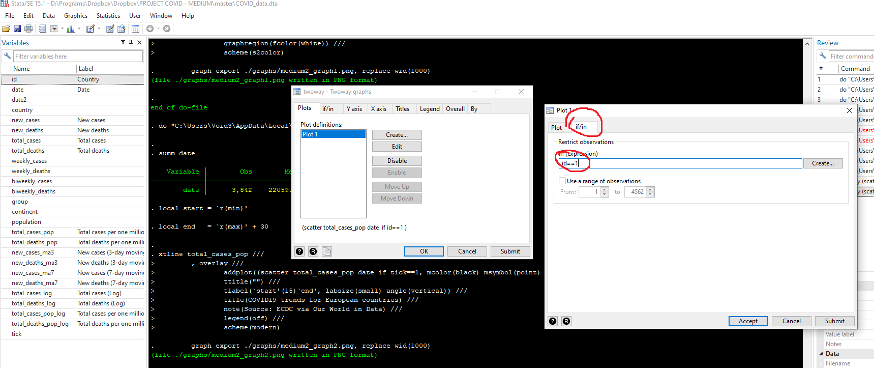
If you press submit, you will get the following syntax and graph:

如果按提交，您将获得以下语法和图形：

twoway /// (line total_cases_pop date if id==1) /// , legend(off) graph export ./graphs/medium2_graph5.png, replace wid(1000)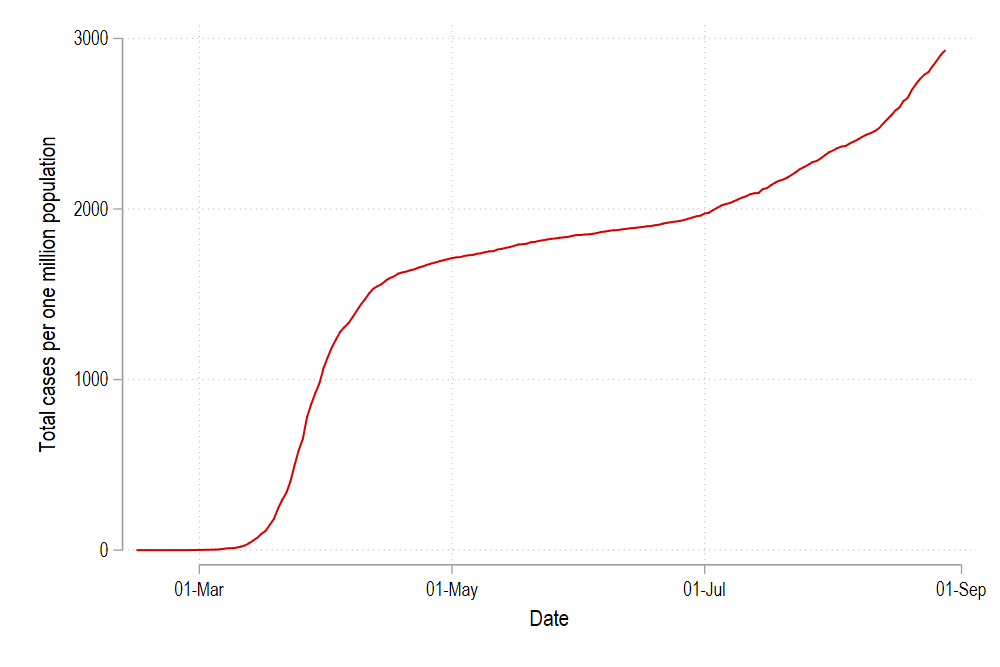

Which gives us just one line in the cleanplots color scheme for the country with id = 1. We can modify this line by changing the color and the line pattern simply by typing:

这给我们提供了id = 1的国家的cleanplots配色方案中的一行。我们可以通过简单地键入以下内容来更改颜色和线条图案来修改该线条：

twoway /// (line total_cases_pop date if id==1, lcolor(green) lpattern(dash)) /// , legend(off)graph export ./graphs/medium2_graph6.png, replace wid(1000)

or we can abbreviate the syntax a bit (where lc = line color, and lp = line pattern, and lw = line width):

或者我们可以稍微简化一下语法(其中lc =线条颜色， lp =线条图案， lw =线条宽度)：

twoway /// (line total_cases_pop date if id==1, lc(green) lp(solid)) /// , legend(off)  graph export ./graphs/medium2_graph7.png, replace wid(1000)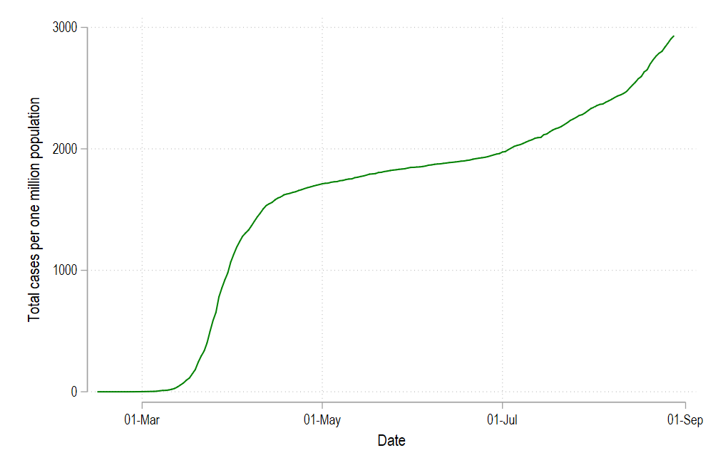

We can add more lines as well by modifying the code above and give the new lines green, blue, and red colors:

我们还可以通过修改上面的代码来添加更多行，并将新行赋予绿色，蓝色和红色：

twoway /// (line total_cases_pop date if id==1, lc(green) lp(solid)) /// (line total_cases_pop date if id==2, lc(blue) lp(solid)) /// (line total_cases_pop date if id==3, lc(red) lp(solid)) /// , legend(off)  graph export ./graphs/medium2_graph8.png, replace wid(1000)

And we can add additional elements to neatly label this graph:

我们可以添加其他元素来整齐地标记此图：

summ datelocal start = `r(min)'local end   = `r(max)' + 30twoway /// (line total_cases_pop date if id==1, lc(green) lp(solid)) /// (line total_cases_pop date if id==2, lc(blue) lp(solid)) /// (line total_cases_pop date if id==3, lc(red) lp(solid)) /// (scatter total_cases_pop date if tick==1 & id <= 3, mcolor(black) msymbol(point) mlabel(country) mlabsize(vsmall) mlabcolor(black)) /// , ///  xlabel(`start'(15)`end', labsize(small) angle(vertical)) ///  legend(off) graph export ./graphs/medium2_graph9.png, replace wid(1000)

In Stata colors can also be defined using RGB values. So for the graph above, the corresponding RGB values for the three graphs:

在Stata中，还可以使用RGB值定义颜色。 因此，对于上面的图形，三个图形的相应RGB值：

Red = “255 0 0”

红色=“ 255 0 0”

Green = “0 128 0”

绿色=“ 0 128 0”

Blue = “0 0 255”

蓝色=“ 0 0 255”

summ datelocal start = `r(min)'local end   = `r(max)' + 30twoway /// (line total_cases_pop date if id==1, lc("255 0 0") lp(solid)) /// (line total_cases_pop date if id==2, lc("0 128 0") lp(solid)) /// (line total_cases_pop date if id==3, lc("0 0 255") lp(solid)) /// (scatter total_cases_pop date if tick==1 & id <= 3, mcolor(black) msymbol(point) mlabel(country) mlabsize(vsmall) mlabcolor(black)) /// , ///  xlabel(`start'(15)`end', labsize(small) angle(vertical)) ///  legend(off) graph export ./graphs/medium2_graph10.png, replace wid(1000)

which gives us exactly the same graph as above:

这给了我们与上面完全相同的图：

We can keep adding new lines and new colors as well, but this quickly becomes inefficient especially if we have a lot of countries. Manually defining a color for each line requires a lot of copy pasting and defining colors for each line.

我们也可以不断添加新的线条和新的颜色，但是这很快变得效率低下，尤其是在我们有很多国家的情况下。 手动为每行定义颜色需要大量复制粘贴并为每行定义颜色。

In order to proceed further, we will work on two new elements:

为了进一步进行，我们将研究两个新元素：

• Using color palettes to replace colors for individual lines使用调色板替换单个线条的颜色
• Generating loops to generate lines for all countries生成循环以生成所有国家/地区的线路

步骤4：使用调色板 (Step 4: Using color palettes)

Here we install two packages written by Benn Jann called palettes and colrspace:

以书面形式在这里，我们安装两个包鸭舌Jann称为调色板和colrspace：

ssc install palettes, replace    // for color palettesssc install colrspace, replace   // for expanding the color base

One can also directly install from Github to make sure we have the very latest update:

也可以从Github直接安装以确保我们具有最新更新：

net install palettes, replace from("https://raw.githubusercontent.com/benjann/palettes/master/")net install colrspace, replace from("https://raw.githubusercontent.com/benjann/colrspace/master/")

The documentation of these packages can be checked here and one can also explore them by typing:

这些软件包的文档可以在此处检查，也可以通过键入以下内容进行探索：

help colorpalettehelp colrspace

Here we will not go into detail of the color theory, or the use of colors since this requires a whole guide on its own. But we will make use of the set of color schemes that come bundled with these packages. For example, colorpalette introduces the popular matplotlib color scheme typically used in R and Python graphs:

在这里，我们将不详细介绍颜色理论或颜色的使用，因为这需要单独的完整指南。 但是，我们将利用这些软件包随附的一组配色方案。 例如，colorpalette引入了流行的matplotlib配色方案，通常在R和Python图形中使用：

colorpalette plasmacolorpalette infernocolorpalette cividiscolorpalette viridis

The viridis color scheme can be easily recognized since it is one of the most used schemes in Python and R (e.g. in ggplots2). We can also generate different color ranges:

翠绿配色方案很容易识别，因为它是Python和R中最常用的配色方案之一(例如ggplots2)。 我们还可以生成不同的颜色范围：

colorpalette viridis, n(10)colorpalette: viridis, n(5) / viridis, n(10) / viridis, n(15)

where the last command gives us:

最后一条命令给我们的位置：

Here we can give whatever value of n to generate a linearly interpolated colors. In the next step, we incorporate the viridis color scheme in the 3 line graph we generate above:

在这里，我们可以给出n的任何值来生成线性插值的颜色。 下一步，我们将viridis配色方案合并到上面生成的3条线图中：

colorpalette viridis, n(3) nograph    // 3 colors and no graphreturn list                          // return the locals stored

The Stata window will show the following output. The key locals for us are r(p1), r(p2), r(p3), which contains the RGB code for the three colors we need to modify the graph. Now rather than copy pasting the RGB code, we can simply store this information in a set of locals:

Stata窗口将显示以下输出。 我们的主要局部变量是r(p1) ， r(p2) ， r(p3) ，其中包含我们需要修改图形的三种颜色的RGB代码。 现在，我们无需复制粘贴RGB代码，而只需将这些信息存储在一组本地语言中：

colorpalette viridis, n(3) nograph return listlocal color1 = r(p1)local color2 = r(p2)local color3 = r(p3)summ datelocal start = r(min)local end   = r(max) + 30twoway /// (line total_cases_pop date if id==1, lc("`color1'") lp(solid)) /// (line total_cases_pop date if id==2, lc("`color2'") lp(solid)) /// (line total_cases_pop date if id==3, lc("`color3'") lp(solid)) /// (scatter total_cases_pop date if tick==1 & id <= 3, mcolor(black) msymbol(point) mlabel(country) mlabsize(vsmall) mlabcolor(black)) /// , ///  xlabel(`start'(15)`end', labsize(small) angle(vertical)) ///  legend(off) graph export ./graphs/medium2_graph11.png, replace wid(1000)

which gives us this graph:

这给了我们这张图：

and if we are using five countries:

如果我们使用五个国家：

colorpalette viridis, n(5) nograph  return listlocal color1 = r(p1)local color2 = r(p2)local color3 = r(p3)local color4 = r(p4)local color5 = r(p5)summ datelocal start = r(min)local end   = r(max) + 30twoway /// (line total_cases_pop date if id==1, lc("`color1'") lp(solid)) /// (line total_cases_pop date if id==2, lc("`color2'") lp(solid)) /// (line total_cases_pop date if id==3, lc("`color3'") lp(solid)) /// (line total_cases_pop date if id==4, lc("`color4'") lp(solid)) /// (line total_cases_pop date if id==5, lc("`color5'") lp(solid)) /// (scatter total_cases_pop date if tick==1 & id <= 5, mcolor(black) msymbol(point) mlabel(country) mlabsize(vsmall) mlabcolor(black)) /// , ///  xlabel(`start'(15)`end', labsize(small) angle(vertical)) ///  legend(off)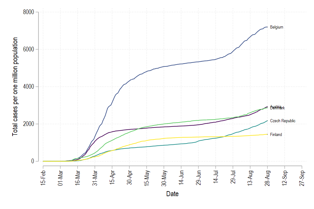

But here we see one problem: the color order is messed up. In order to fix the color graduation, we need to create a rank of countries from lowest to highest values (or vice versa) on the last date (which we have also marked with the variable tick). This can be done in Stata using the egen command:

但是在这里我们看到一个问题：颜色顺序混乱了。 为了修正颜色分级，我们需要在最后一个日期(也用变量tick标记)上创建从最低值到最高值(反之亦然)的国家/地区等级。 这可以使用egen命令在Stata中完成：

egen rank = rank(total_cases_pop) if tick==1, f

Tip: See help egen for a complete list of very useful commands. Also check egenmore which extends the functionality of egen.

提示：有关非常有用的命令的完整列表，请参见help egen 。 还要检查egenmore ，它扩展了egen的功能。

We can see that the correct order has been identified by typing:

我们可以看到通过键入以下命令确定了正确的订单：

sort date rank br country date total_cases_pop rank if tick==1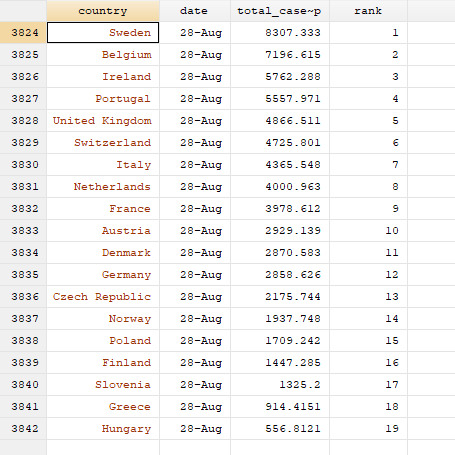

Here we can see that Sweden has the highest cumulative cases per million population and is ranked 1, while Hungary has the lowest cumulative cases per mission population and has a rank of 19.

在这里我们可以看到，瑞典每百万人口的累积病例数最高，排名第1，而匈牙利每特派团人口的累积病例数最低，排名第19。

Now to get the correct colors, this ranking has to be applied to ALL the past observations as well. Here we introduce a level loop:

现在要获得正确的颜色，此排名也必须应用于所有过去的观察结果。 在这里，我们介绍一个级别循环：

levelsof country, local(lvls)foreach x of local lvls { display "`x'" qui summ rank if country=="`x'"  // summarize the rank of country x cap replace rank = `r(max)' if country=="`x'" & rank==. }

Tip: Levels of individual unique elements within a variable. The levelsof command help automating looping over all unique values without having to manually define them.

提示：变量中各个唯一元素的级别。 levelof命令可帮助自动循环所有唯一值，而无需手动定义它们。

The first command levelsof, stores all the unique values of countries in the local lvls. foreach loops over each lvl (see help forheach). The command display shows the country we are currently looping. qui stands for quietly, and it hides displaying the summarize (summ) command in the Stata output window. This is strictly not necessary. replace replaces the rank variable with the max value returned from the summarize command above for each country and for all empty observations. The capture command (cap), effectively skips the execution of this command if an error occurs. This is a powerful command that allows us to bypass code errors. Errors stop the executing of the code and display an error. capture should only be used if you know exactly what you are doing. The reason we use it here, is because one country (Spain) does not have an observation for the last date. Hence the summarize command returns nothing and therefore there is nothing to be replaced. We can fine tune this code, but this requires adding additional elements not necessary for this guide. We will leave it for other guides in the future.

第一个命令levelof ，将国家的所有唯一值存储在本地lvls中 。 foreach在每个lvl上循环(请参阅help forheach) 。 命令显示将显示我们当前正在循环播放的国家/地区。 qui安静地代表，它隐藏在Stata输出窗口中显示summary ( summ )命令。 完全没有必要。 replace将上述变量替换为上面的summary命令为每个国家和所有空观测值返回的最大值的等级变量。 如果发生错误，那么捕获命令( cap )有效地跳过该命令的执行。 这是一个功能强大的命令，可让我们绕过代码错误。 错误会停止执行代码并显示错误。 仅当您确切知道自己在做什么时，才应使用捕获 。 我们在这里使用它的原因是因为一个国家(西班牙)没有最后日期的观测值。 因此，summary命令不返回任何内容，因此没有任何要替换的内容。 我们可以对此代码进行微调，但这需要添加本指南中不必要的其他元素。 将来我们会将其留给其他指南使用。

Once the ranks are defined, we now generate the graph again, BUT, this time we do not plot on the variable id, but on the variable rank:

定义等级后，我们现在再次生成图形，但这次，我们不会在变量id上绘制，而是在变量等级上绘制：

colorpalette viridis, n(5) nograph  return listlocal color1 = r(p1)local color2 = r(p2)local color3 = r(p3)local color4 = r(p4)local color5 = r(p5)summ datelocal start = r(min)local end   = r(max) + 30twoway /// (line total_cases_pop date if rank==1, lc("`color1'") lp(solid)) /// (line total_cases_pop date if rank==2, lc("`color2'") lp(solid)) /// (line total_cases_pop date if rank==3, lc("`color3'") lp(solid)) /// (line total_cases_pop date if rank==4, lc("`color4'") lp(solid)) /// (line total_cases_pop date if rank==5, lc("`color5'") lp(solid)) /// (scatter total_cases_pop date if tick==1 & rank <= 5, mcolor(black) msymbol(point) mlabel(country) mlabsize(vsmall) mlabcolor(black)) /// , ///  xlabel(`start'(15)`end', labsize(small) angle(vertical)) ///  legend(off)  graph export ./graphs/medium2_graph13.png, replace wid(1000)

which gives us:

这给了我们：

Since the variables id and rank are not the same, we get a different set of countries. But the main thing here is that all lines are colored in the correct order.

由于变量id和rank不相同，因此我们得到了一组不同的国家。 但是这里最主要的是所有行都按正确的顺序着色。

步骤5：全自动 (Step 5: Full automation)

Now we come to trickiest part of the code: adding all the countries and generating their corresponding colors. Here the code will get fairly complex, but we will go over the logic step-by-step.

现在我们来看代码中最棘手的部分：添加所有国家/地区并生成其相应的颜色。 这里的代码将变得相当复杂，但我们将逐步讲解逻辑。

First, lines cannot be added manually for each country. Especially if we are using different country groupings with different number of countries. Stata, by default, has no option of batch modifying lines in graphs. This is probably only possible in the panel data, xtline command but it also has limited functionality when it comes to modifying the elements of each line. In order to bypass this limitation, what we can do is generate the graph command using locals and loops. If we look at the graph commands above, there is a pattern to how the lines are generated:

首先，不能为每个国家/地区手动添加行。 尤其是当我们使用不同国家/地区的不同国家/地区分组时。 默认情况下，Stata不能批量修改图形中的线。 这可能仅在面板数据xtline命令中可行，但在修改每行的元素时功能也有限。 为了绕过此限制，我们可以做的是使用局部变量和循环生成graph命令。 如果我们看一下上面的graph命令，将有一条直线生成方式：

(line total_cases_pop date if rank==1, lc("`color1'") lp(solid)) ///(line total_cases_pop date if rank==2, lc("`color2'") lp(solid)) ///

First line says rank = 1 and lc(..color1..), second line says rank=2 and color2 etc. Thus the numbers define both the rank and the color value. Hence, if we know the total number of countries, we can loop over them and sequentially generate code for each line.

第一行表示等级= 1和lc(.. color1 ..)，第二行表示等级= 2和color2等。因此，数字定义了等级和颜色值。 因此，如果我们知道国家/地区的总数，则可以遍历国家/地区并为每一行依次生成代码。

Since this is a non-standard Stata graph procedure, I will give the code for looping over the total observations and generating these lines:

由于这是一个非标准的Stata图过程，因此我将给出用于遍历总观测值并生成以下行的代码：

levelsof rank, local(lvls)   // loop over all the levelslocal items = r(r)           // pick the total items foreach x of local lvls { colorpalette viridis, n(`items') nograph local customline `customline' (line total_cases_pop date if rank == `x', lc("`r(p`x')'") lp(solid)) ||  }

and discuss it here:

并在这里讨论：

levelsof generates the unique values of rank, which also equals the number of countries (each country has a unique rank). local items store the total number of unique rank values for use later. foreach loops over all the rank levels. For each level, a colorpalette for the viridis color scheme is generated for the number of countries defined in the local items.

levelof生成唯一的等级值，也等于国家/地区的数量(每个国家/地区都有唯一的等级)。 本地项目存储唯一等级值的总数，以供以后使用。 foreach在所有等级上循环。 对于每个级别，将针对本地项目中定义的国家/地区数量生成viridis配色方案的调色板 。

The next command stores the information for each rank in local called customline. Every time the loop goes on to the next rank value, the information of the new line graph is appended to the existing line. Each line is given a color value r(px), where x is the rank order and r(px) is the corresponding color value from the colorpalette for that specific rank.

下一条命令将每个等级的信息存储在本地称为customline的行中。 每当循环继续到下一个等级值时，新折线图的信息就会附加到现有折线上。 每行都有一个颜色值r(p x )，其中x是等级顺序，r(p x )是该特定等级的调色板中对应的颜色值。

Note that this type of programming is fairly common in softwares like Matlab, Mathematica, and R as well which mostly work with lists and matrices.

请注意，这种类型的编程在Matlab，Mathematica和R等软件中也很常见，这些软件主要用于列表和矩阵。

The double pipe command (||), is Stata’s internal command for splitting line graphs. Essentially the local customline contains information on all the lines for all the countries. This can be used as follows:

双管道命令(||)是Stata的内部折线图命令。 本质上，本地定制行包含有关所有国家/地区的所有行的信息。 可以如下使用：

levelsof rank, local(lvls)   // loop over all the levelslocal items = r(r)foreach x of local lvls { colorpalette viridis, n(`items') nographlocal customline `customline' (line total_cases_pop date if rank == `x', lc("`r(p`x')'") lp(solid)) ||  }summ datelocal start = r(min)local end   = r(max) + 30twoway `customline' /// (scatter total_cases_pop date if tick==1 & rank <= `items', mcolor(black) msymbol(point) mlabel(country) mlabsize(vsmall) mlabcolor(black)) /// , ///  xlabel(`start'(15)`end', labsize(small) angle(vertical)) ///  xtitle("") ///  title("COVID-19 trends for European countries") ///  note("Source: ECDC via Our World in Data", size(vsmall)) ///  legend(off) graph export ./graphs/medium2_graph_final.png, replace wid(1000)

Which gives us this neat looking graph:

这给了我们这个整洁的图形：

The code above can be used with any number of lines to auto color and label the line graphs. This logic of loop and automation of code can also be used for any complex operation involving different groups and different level sizes.

上面的代码可与任意数量的线一起使用，以自动为线图着色和标记。 这种循环逻辑和代码自动化也可以用于涉及不同组和不同级别大小的任何复杂操作。

行使 (Exercise)

Try generating the graph with different a country grouping and another color scheme.

尝试使用其他国家/地区分组和另一种配色方案生成图形。

其他指南 (Other guides)

Part 1: An introduction to data setup and customized graphs

第1部分：数据设置和自定义图的介绍

Part 2: Customizing colors schemes

第2部分：自定义配色方案

Part 3: Heat plots

第3部分：热图

If you enjoy these guides and find them useful, then please like and follow my Medium Stata blog: <do> The Stata Guide

如果您喜欢这些指南并发现它们很有用，请喜欢并关注我的Medium Stata博客： <do> Stata指南

关于作者 (About the author)

I am an economist by profession and I have been using Stata for almost 18 years. I have worked and lived across three different continents. I am currently based in Vienna, Austria. You can find my research work on ResearchGate and codes repository on GitHub. You can follow my COVID-19 related Stata visualizations on my Twitter. I am also featured on the COVID19 Stata webpage in the visualization and graphics section.

我是一名经济学家，并且已经使用Stata近18年了。 我曾在三个不同的大陆工作和生活过。 我目前居住在奥地利维也纳。 您可以在ResearchGate和GitHub上的代码存储库中找到我的研究工作。 您可以在Twitter上关注与COVID-19相关的Stata可视化。 我还出现在COVID19 Stata网页的“可视化和图形”部分中。

You can connect with me via Medium, Twitter, LinkedIn or simply through email: asjadnaqvi@gmail.com.

您可以通过Medium ， Twitter ， LinkedIn或通过电子邮件与我们联系：asjadnaqvi@gmail.com。

My Medium blog for Stata stories here: <do> The Stata Guide

我的Stata故事我的中型博客： <do> Stata指南