altair 8800_Python数据可视化场景的戏剧性浏览（包括ggpy和Altair）

altair 8800

由Dan Saber | 2017年4月19日 (by Dan Saber | April 19, 2017)

This post originally appeared on Dan Saber’s blog. We thought it was hilarious, so we asked him if we could repost it. He generously agreed!

该帖子最初出现在Dan Saber的博客上。我们认为这很有趣，所以我们问他是否可以重新发布它。他慷慨地同意了！

About Dan: My name is Dan Saber. I’m a UCLA math grad, and I do Data Science at Coursera. (Before that, I worked in Finance.) I love writing, music, programming, and — despite the American education system’s best attempts — statistics.

关于丹 ：我叫丹·萨伯。我是UCLA数学专业的毕业生，我在Coursera从事数据科学专业。（在此之前，我曾在财务部门工作。）我喜欢写作，音乐，编程，尽管美国教育系统已尽力，但我还是喜欢统计学。

为什么要尝试，老兄？ (Why Even Try, Man?)

I recently came upon Brian Granger and Jake VanderPlas’s Altair, a promising young visualization library. Altair seems well-suited to addressing Python’s ggplot envy, and its tie-in with JavaScript’s Vega-Lite grammar means that as the latter develops new functionality (e.g., tooltips and zooming), Altair benefits — seemingly for free!

我最近遇到了Brian Granger和Jake VanderPlas的Altair，这是一个很有前途的年轻可视化库。 Altair似乎非常适合解决Python的ggplot羡慕问题，它与JavaScript的Vega-Lite语法相结合意味着，随着后者开发新功能（例如，工具提示和缩放），Altair受益-似乎是免费的！

Indeed, I was so impressed by Altair that the original thesis of my post was going to be: “Yo, use Altair.”

确实，我对Altair印象深刻，以至于我帖子的原始主题是：“哦，使用Altair。”

But then I began ruminating on my own Pythonic visualization habits, and — in a painful moment of self-reflection — realized I’m all over the place: I use a hodgepodge of tools and disjointed techniques depending on the task at hand (usually whichever library I first used to accomplish that task¹).

但是后来我开始反思自己的Pythonic可视化习惯，并且-在痛苦的自我反省中-意识到我无所不在：我根据手头的任务使用各种工具和不连贯的技术（通常以我首先用来完成该任务的库¹ ）。

This is no good. As the old saying goes: “The unexamined plot is not worth exporting to a PNG.”

不好俗话说：“未经检查的地块不值得出口到巴布亚新几内亚。”

Thus, I’m using my discovery of Altair as an opportunity to step back — to investigate how Python’s statistical visualization options hang together. I hope this investigation proves helpful for you as well.

因此，我将自己对Altair的发现作为回退的机会-研究Python的统计可视化选项如何组合在一起。希望这项调查对您也有所帮助。

怎么样了？ (How’s This Gonna Go?)

The conceit of this post will be: “You need to do Thing X. How would you do Thing X in matplotlib? pandas? Seaborn? ggpy? Altair?” By doing many different Thing X’s, we’ll develop a reasonable list of pros, cons, and takeaways — or at least a whole bunch of code that might be somehow useful.

这篇文章的自负是：“您需要做ThingX。如何在matplotlib中做Thing X？大熊猫？ Seaborn？ ggpy？牵牛星？” 通过执行许多不同的Thing X，我们将开发一个合理的利弊清单，或者至少是一堆有用的代码。

(Warning: this all may happen in the form of a two-act play.)

（警告：这一切都可能以两幕剧的形式发生。）

选项（以主观复杂性的降序排列） (The Options (in ~Descending Order of Subjective Complexity))

First, let’s welcome our friends²:

首先，欢迎我们的朋友² ：

matplotlib (matplotlib)

The 800-pound gorilla — and like most 800-pound gorillas, this one should probably be avoided unless you genuinely need its power, e.g., to make a custom plot or produce a publication-ready graphic.

800磅的大猩猩-和大多数800磅的大猩猩一样，除非您真正需要它的功能，例如制作自定义图或准备出版的图形，否则应该避免使用这种大猩猩。

(As we’ll see, when it comes to statistical visualization, the preferred tack might be: “do as much as you easily can in your convenience layer of choice [i.e., any of the next four libraries], and then use matplotlib for the rest.”)

（如我们将看到的，在统计可视化方面，首选的方法可能是：“在您选择的便利层中（即接下来的四个库中的任何一个）轻松地做很多，然后使用matplotlib其余的部分。”）

大熊猫 (pandas)

“Come for the DataFrames; stay for the plotting convenience functions that are arguably more pleasant than the matplotlib code they supplant.” — rejected pandas taglines

“为数据框架而来；保留绘图便利功能，可以说比它们取代的matplotlib代码更令人愉快。” -被拒绝的熊猫标语

(Bonus tidbit: the pandas team must include a few visualization nerds, as the library includes things like RadViz plots and Andrews Curves that I haven’t seen elsewhere.)

（奖金花絮：熊猫团队必须包括一些可视化的书呆子，因为该库包含RadViz绘图和Andrews Curves之类的东西，而我在其他地方没有看到过。）

海生 (Seaborn)

Seaborn has long been my go-to library for statistical visualization; it summarizes itself thusly:

长期以来，Seaborn一直是我进行统计可视化的首选库；因此总结如下：

“If matplotlib ‘tries to make easy things easy and hard things possible,’ seaborn tries to make a well-defined set of hard things easy too”

“如果matplotlib'试图使容易的事情变得容易而使困难的事情变得可能，'seaborn也会尝试使一组定义明确的困难的事情也变得容易”

yhat的ggpy (yhat’s ggpy)

A Python implementation of the wonderfully declarative ggplot2. This isn’t a “feature-for-feature port of ggplot2,” but there’s strong feature overlap. (And speaking as a part-time R user, the main geoms seem to be in place.)

出色的声明性ggplot2的Python实现。这不是“ ggplot2的功能对端口”，但是功能上有很多重叠之处。（以兼职R用户的身份讲，主要地理元素似乎就位。）

牵牛星 (Altair)

The new guy, Altair is a “declarative statistical visualization library” with an exceedingly pleasant API.

新人Altair是一个“声明式统计可视化库”，具有非常令人愉悦的API。

Wonderful. Now that our guests have arrived and checked their coats, let’s settle in for our very awkward dinner conversation. Our show is entitled…

精彩。现在我们的客人已经到达并检查了他们的外套，让我们安顿下来，进行我们非常尴尬的晚餐对话。我们的节目的标题是……

Python可视化库的小商店（由所有库自己担任主角） (Little Shop of Python Visualization Libraries (starring all libraries as themselves))

ACT I：线条和点 (ACT I: LINES AND DOTS)

(In Scene 1, we’ll be dealing with a tidy data set named “ts.” It consists of three columns: a “dt” column (for dates); a “value” column (for values); and a “kind” column, which has four unique levels: A, B, C, and D. Here’s a preview…)

（在场景1中，我们将处理一个名为“ ts”的整洁数据集。它由三列组成：“ dt”列（用于日期）；“ value”列（用于值）；以及“种类” ”列，它具有四个独特的级别：A，B，C和D。这是预览…）

		dt	dt	kind	类	value	值
0	0	2000-01-01	2000-01-01	A	一个	1.442521	1.442521
1	1个	2000-01-02	2000-01-02	A	一个	1.981290	1.981290
2	2	2000-01-03	2000-01-03	A	一个	1.586494	1.586494
3	3	2000-01-04	2000-01-04	A	一个	1.378969	1.378969
4	4	2000-01-05	2000-01-05	A	一个	-0.277937	-0.277937

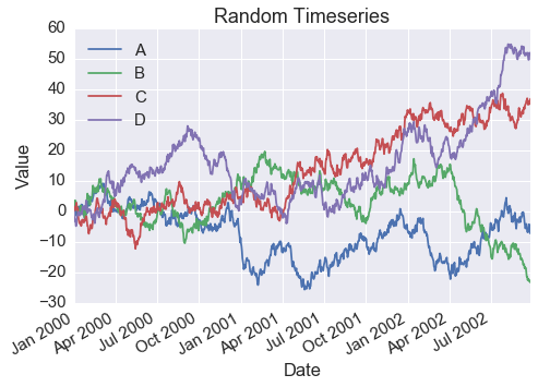
场景1：如何在同一张图上绘制多个时间序列？ (Scene 1: How would you plot multiple time series on the same graph?)

matplotlib: Ha! Haha! Beyond simple. While I could and would accomplish this task in any number of complex ways, I know your feeble brains would crumble under the weight of their ingenuity. Hence, I dumb it down, showing you two simple methods. In the first, I loop through your trumped-up matrix — I believe you peons call it a “Data” “Frame” — and subset it to the relevant time series. Next, I invoke my “plot” method and pass in the relevant columns from that subset.

matplotlib ：哈！哈哈！超越简单。尽管我可以而且将以多种复杂的方式完成这项任务，但我知道您的软弱的大脑会在他们的聪明才智的重压下崩溃。因此，我将其简化，向您展示了两种简单的方法。首先，我循环浏览您的重要矩阵（我相信您的工具将其称为“数据”“框架”），并将其子集化为相关的时间序列。接下来，我调用我的“绘图”方法，并从该子集中传入相关的列。

# MATPLOTLIB
fig, ax = plt.subplots(1, 1,
figsize=(7.5, 5))
for k in ts.kind.unique():
tmp = ts[ts.kind == k]
ax.plot(tmp.dt, tmp.value, label=k)
ax.set(xlabel='Date',
ylabel='Value',
title='Random Timeseries')
ax.legend(loc=2)
fig.autofmt_xdate()

# MATPLOTLIB
fig, ax = plt.subplots(1, 1,
figsize=(7.5, 5))
for k in ts.kind.unique():
tmp = ts[ts.kind == k]
ax.plot(tmp.dt, tmp.value, label=k)
ax.set(xlabel='Date',
ylabel='Value',
title='Random Timeseries')
ax.legend(loc=2)
fig.autofmt_xdate()

MPL: Next, I enlist this chump (motions to pandas), and have him pivot this “Data” “Frame” so that it looks like this…

MPL ：接下来，我征集这个怪人（向熊猫运动），并让他枢转这个“数据”“框架”，使其看起来像这样……

kind	类	A	一个	B	乙	C	C	D	d
dt	dt
2000-01-01	2000-01-01	1.442521	1.442521	1.808741	1.808741	0.437415	0.437415	0.096980	0.096980
2000-01-02	2000-01-02	1.981290	1.981290	2.277020	2.277020	0.706127	0.706127	-1.523108	-1.523108
2000-01-03	2000-01-03	1.586494	1.586494	3.474392	3.474392	1.358063	1.358063	-3.100735	-3.100735
2000-01-04	2000-01-04	1.378969	1.378969	2.906132	2.906132	0.262223	0.262223	-2.660599	-2.660599
2000-01-05	2000-01-05	-0.277937	-0.277937	3.489553	3.489553	0.796743	0.796743	-3.417402	-3.417402

MPL: By transforming the data into an index with four columns — one for each line I want to plot — I can do the whole thing in one fell swoop (i.e., a single call of my “plot” function).

MPL ：通过将数据转换为具有四列的索引（我要绘制的每一行一个索引），我可以一口气完成全部工作（即，一次调用“ plot”函数）。

# MATPLOTLIB
fig, ax = plt.subplots(1, 1,
figsize=(7.5, 5))
ax.plot(dfp)
ax.set(xlabel='Date',
ylabel='Value',
title='Random Timeseries')
ax.legend(dfp.columns, loc=2)
fig.autofmt_xdate()

# MATPLOTLIB
fig, ax = plt.subplots(1, 1,
figsize=(7.5, 5))
ax.plot(dfp)
ax.set(xlabel='Date',
ylabel='Value',
title='Random Timeseries')
ax.legend(dfp.columns, loc=2)
fig.autofmt_xdate()

pandas (looking timid): That was great, Mat. Really great. Thanks for including me. I do the same thing — hopefully as good? (smiles weakly)

熊猫（看上去很胆小）：太好了，马特。非常好。谢谢包括我。我做同样的事情-希望一样好吗？（微弱地微笑）

pandas: It looks exactly the same, so I just won’t show it.

熊猫：看起来完全一样，所以我不会显示。

Seaborn (smoking a cigarette and adjusting her beret): Hmmm. Seems like an awful lot of data manipulation for a silly line graph. I mean, for loops and pivoting? This isn’t the 90’s or Microsoft Excel. I have this thing called a FacetGrid I picked up when I went abroad. You’ve probably never heard of it…

Seaborn （抽烟并调整贝雷帽）：嗯。愚蠢的折线图似乎需要大量的数据处理。我的意思是，要循环和旋转吗？这不是90年代或Microsoft Excel。我有一个叫做FacetGrid的东西，我出国时就接了。您可能从未听说过……

# SEABORN
g = sns.FacetGrid(ts, hue='kind', size=5, aspect=1.5)
g.map(plt.plot, 'dt', 'value').add_legend()
g.ax.set(xlabel='Date',
ylabel='Value',
title='Random Timeseries')
g.fig.autofmt_xdate()

# SEABORN
g = sns.FacetGrid(ts, hue='kind', size=5, aspect=1.5)
g.map(plt.plot, 'dt', 'value').add_legend()
g.ax.set(xlabel='Date',
ylabel='Value',
title='Random Timeseries')
g.fig.autofmt_xdate()

SB: See? You hand FacetGrid your un-manipulated tidy data. At that point, passing in “kind” to the “hue” parameter means you’ll plot four different lines — one for each level in the “kind” field. The way you actually realize these four different lines is by mapping my FacetGrid to this Philistine’s (motions to matplotlib) plot function, and passing in “x” and “y” arguments. There are some things you need to keep in mind, obviously, like manually adding a legend, but nothing too challenging. Well, nothing too challenging for some of us…

SB ：看到了吗？您将FacetGrid交给您未处理的整齐数据。届时，将“ kind”传递给“ hue”参数意味着您将绘制四条不同的线-“ kind”字段中每个级别对应一条线。实际实现这四行不同的方式是，将我的FacetGrid映射到该Philistine的（向matplotlib传递的运动）绘图函数，并传递“ x”和“ y”参数。显然，您需要记住一些事情，例如手动添加图例，但是没有什么太具挑战性。好吧，对于我们中的某些人来说，没有什么挑战性……

ggpy: Wow, neat! I do something similar, but I do it like my big bro. Have you heard of him? He’s so coo–

ggpy ：哇，整洁！我做类似的事情，但是我做得像我的大哥。你听说过他吗？他很酷

SB: Who invited the kid?

SB ：谁邀请了这个孩子？

GG: Check it out!

GG ：看看！

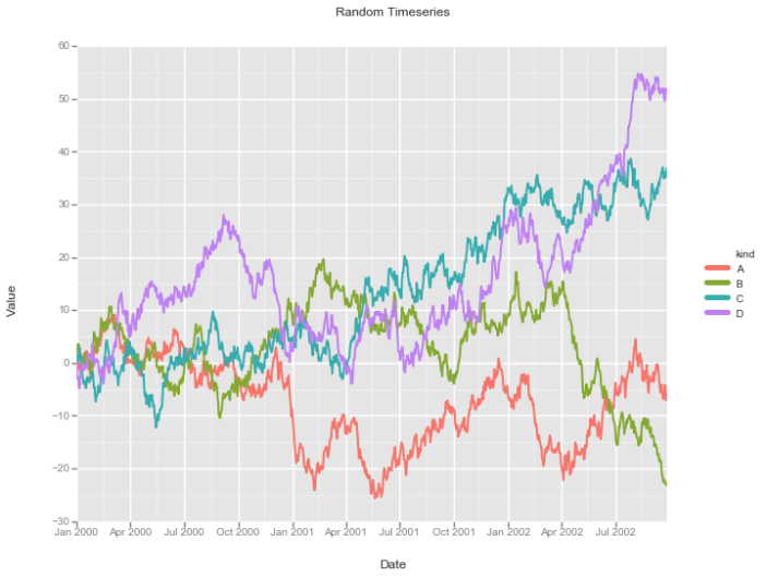
GG: (picks up ggplot2 by Hadley Wickham and sounds out words): Every plot is com — com — com-prised of data (e.g., “ts”), aesthetic mappings (e.g, “x”, “y”, “color”), and the geometric shapes that turn our data and aesthetic mappings into a real visualization (e.g., “geom_line”)!

GG ：（由Hadley Wickham挑选ggplot2并发声）：每个图都是com — com —包括数据（例如“ ts”），美学映射（例如“ x”，“ y”，“颜色”） ”），以及将我们的数据和美学映射转变为真实可视化效果的几何形状（例如“ geom_line”）！

Altair: Yup, I do that, too.

Altair ：是的，我也这样做。

# ALTAIR
c = Chart(ts).mark_line().encode(
x='dt',
y='value',
color='kind'
)
c

# ALTAIR
c = Chart(ts).mark_line().encode(
x='dt',
y='value',
color='kind'
)
c

ALT: You give my Chart class some data and tell it what kind of visualization you want: in this case, it’s “mark_line”. Next, you specify your aesthetic mappings: our x-axis needs to be “date”; our y-axis needs to be “value”; and we want to split by kind, so we pass “kind” to “color.” Just like you, GG (tousles GG’s hair). Oh, and by the way, using the same color scheme y’all use isn’t a problem, either:

ALT ：您给我的Chart类一些数据，并告诉它您想要哪种可视化效果：在这种情况下，它是“ mark_line”。接下来，您指定美学映射：我们的x轴需要为“日期”；我们的y轴必须是“值”；并且我们想按种类拆分，因此我们将“种类”传递给“颜色”。就像您一样，GG（GG的尾巴）。哦，顺便说一句，使用相同的配色方案，所有使用都不是问题，或者：

MPL stares in terrified wonder

MPL惊恐万分

分析场景1 (Analyzing Scene 1)

Aside from matplotlib being a jerk³, a few themes emerged:

除了matplotlib混蛋^3之外，还出现了一些主题：

In matplotlib and pandas, you must either make multiple calls to the “plot” function (e.g., once-per-for loop), or you must manipulate your data to make it optimally fit the plot function (e.g., pivoting). (That said, there’s another technique we’ll see in Scene 2.)
(To be frank, I never used to think this was a big deal, but then I met people who use R. They looked at me aghast.)
Conversely, ggpy and Altair implement similar and declarative “grammar of graphics”-approved ways to handle our simple case: you give their “main” function– “ggplot” in ggpy and “Chart” in Altair” — a tidy data set. Next, you define a set of aesthetic mappings — x, y, and color — that explain how the data will map to our geoms (i.e., the visual marks that do the hard work of conveying information to the reader). Once you actually invoke said geom (“geom_line” in ggpy and “mark_line” in Altair), the data and aesthetic mappings are transformed into visual ticks that a human can understand — and thus, an angel gets its wings.
Intellectually, you can — and probably should (?) — view Seaborn’s FacetGrid through the same lens; however, it’s not 100% identical. FacetGrid needs a hue argument upfront — alongside your data — but wants the x and y arguments later. At that point, your mapping isn’t an aesthetic one, but a functional one: for each “hue” in your data set, you’re simply calling matplotlib’s plot function using “dt” and “value” as its x and y arguments. The for loop is simply hidden from you.
That said, even though the aesthetic maps happen in two separate steps, I prefer the aesthetic mapping mindset to the imperative mindset (at least when it comes to plotting).

在matplotlib和pandas中，您必须多次调用“ plot”函数（例如，每次循环一次），或者必须操纵数据以使其最佳地适合plot函数（例如，旋转）。（也就是说，我们将在场景2中看到另一种技术。）
（坦率地说，我以前从未认为这有什么大不了，但是后来我遇到了使用R的人。他们看着我很震惊。）
相反，ggpy和Altair实现了类似且声明性的“图形语法”批准的方式来处理我们的简单情况：给它们的“主要”功能-ggpy中的“ ggplot”和Altair中的“ Chart”（整洁的数据集）。接下来，您定义了一组美学映射（x，y和颜色），它们解释了数据将如何映射到我们的地理区域（即，视觉标记，这些标记完成向读者传达信息的艰苦工作）。一旦您实际调用了所说的geom（在ggpy中为“ geom_line”，在Altair中为“ mark_line”），数据和美学映射便转换为人类可以理解的视觉标记，从而使天使振翅高飞。
从理智上讲，您可以并且可能应该（？）通过同一镜头查看Seaborn的FacetGrid。但是，它不是100％相同。 FacetGrid需要预先将色相参数与数据一起使用，但稍后需要x和y参数。那时，您的映射不是一种美学的映射，而是一种实用的映射：对于数据集中的每个“色相”，您只需使用“ dt”和“ value”作为其x和y参数调用matplotlib的plot函数。 for循环只是对您隐藏了。
就是说，尽管美学图是分两个步骤进行的，但我更喜欢美学映射的思维方式而不是命令式的思维方式（至少在绘图方面）。

Data Aside

暂存数据

(In Scenes 2-4, we’ll be dealing with the famous “iris” data set [though we refer to it as “df” in our code]. It consists of four numeric columns corresponding to various measurements, and a categorical column corresponding to one of three species of iris. Here’s a preview…)

（在场景2-4中，我们将处理著名的“ iris”数据集（尽管在我们的代码中将其称为“ df”）。它由四个分别对应于各种度量的数字列和一个分类列组成对应三种虹膜之一。以下是预览...）

		petalLength	花瓣长度	petalWidth	花瓣宽度	sepalLength	sepalLength	sepalWidth	sepalWidth	species	种类
0	0	1.4	1.4	0.2	0.2	5.1	5.1	3.5	3.5	setosa	Setosa
1	1个	1.4	1.4	0.2	0.2	4.9	4.9	3.0	3.0	setosa	Setosa
2	2	1.3	1.3	0.2	0.2	4.7	4.7	3.2	3.2	setosa	Setosa
3	3	1.5	1.5	0.2	0.2	4.6	4.6	3.1	3.1	setosa	Setosa
4	4	1.4	1.4	0.2	0.2	5.0	5.0	3.6	3.6	setosa	Setosa

场景2：如何绘制散点图？ (Scene 2: How would you make a scatter plot?)

MPL (looking shaken): I mean, you could do the for loop thing again. Of course. And that would be fine. Of course. See? (lowers voice to a whisper) Just remember to set the color argument explicitly or else the dots will all be blue…

MPL （看起来很动摇）：我的意思是，您可以再次执行for循环操作。当然。那很好。当然。看到？（将声音降低到耳语）只需记住显式设置color参数，否则点将全部变为蓝色…

# MATPLOTLIB
fig, ax = plt.subplots(1, 1, figsize=(7.5, 7.5))
for i, s in enumerate(df.species.unique()):
tmp = df[df.species == s]
ax.scatter(tmp.petalLength, tmp.petalWidth,
label=s, color=cp[i])
ax.set(xlabel='Petal Length',
ylabel='Petal Width',
title='Petal Width v. Length -- by Species')
ax.legend(loc=2)

# MATPLOTLIB
fig, ax = plt.subplots(1, 1, figsize=(7.5, 7.5))
for i, s in enumerate(df.species.unique()):
tmp = df[df.species == s]
ax.scatter(tmp.petalLength, tmp.petalWidth,
label=s, color=cp[i])
ax.set(xlabel='Petal Length',
ylabel='Petal Width',
title='Petal Width v. Length -- by Species')
ax.legend(loc=2)

MPL: But, uh, (feigning confidence) I have a better way! Look at this:

MPL ：但是，（充满信心）我有更好的办法！看这个：

MPL: Here, I define a function named “scatter.” It will take groups from a pandas groupby object and plot petal length on the x-axis and petal width on the y-axis. Once per group! Powerful!

MPL ：在这里，我定义了一个名为“ scatter”的函数。它将从熊猫groupby对象中进行分组，并在x轴上绘制花瓣长度，在y轴上绘制花瓣宽度。每组一次！强大！

P: Wonderful, Mat! Wonderful! Essentially what I would have done, so I will sit this one out.

警：太好了，席子！精彩！本质上是我会做的，所以我将把这一部分排除在外。

SB (grinning): No pivoting this time?

SB （笑）：这次没有枢轴吗？

P: Well, in this case, pivoting is complex. We can’t have a common index like we could with our time series data set, and so —

P ：恩，在这种情况下，旋转很复杂。我们无法像时间序列数据集那样拥有共同的索引，因此-

MPL: SHHHHH! WE DON’T HAVE TO EXPLAIN OURSELVES TO HER.

MPL ：嘘！我们不必向她解释自己。

SB: Whatever. Anyway, in my mind, this problem is the same as the last one. Build another FacetGrid but borrow plt.scatter rather than plt.plot.

SB ：随便。无论如何，在我看来，这个问题与上一个相同。构建另一个FacetGrid，但借用plt.scatter而不是plt.plot。

# SEABORN
g = sns.FacetGrid(df, hue='species', size=7.5)
g.map(plt.scatter, 'petalLength', 'petalWidth').add_legend()
g.ax.set_title('Petal Width v. Length -- by Species')

# SEABORN
g = sns.FacetGrid(df, hue='species', size=7.5)
g.map(plt.scatter, 'petalLength', 'petalWidth').add_legend()
g.ax.set_title('Petal Width v. Length -- by Species')

GG: Yes! Yes! Same! You just gotta swap out geom_line for geom_point!

GG ：是的！是! 相同！您只需将geom_line换成geom_point！

ALT (looking bemused): Yup — just swap our mark_line for mark_point.

ALT （看上去很困惑）：是的—只需将我们的mark_line换成mark_point。

# ALTAIR
c = Chart(df).mark_point(filled=True).encode(
x='petalLength',
y='petalWidth',
color='species'
)
c

# ALTAIR
c = Chart(df).mark_point(filled=True).encode(
x='petalLength',
y='petalWidth',
color='species'
)
c

分析场景2 (Analyzing Scene 2)

Here, the potential complications that emerge from building up the API from your data become clearer. While the pandas pivoting trick was extremely convenient for time series, it doesn’t translate so well to this case.
To be fair, the “group by” method is somewhat generalizable, and the “for loop” method is very generalizable; however, they require more custom logic, and custom logic requires custom work: you would need to reinvent a wheel that Seaborn has kindly provided for you.
Conversely, Seaborn, ggpy, and Altair all realize that scatter plots are in many ways line plots without the assumptions (however innocuous those assumptions may be). As such, our code from Scene 1 can largely be reused, but with a new geom (geom_point/mark_point in the case of ggpy/Altair) or a new method (plt.scatter in the case of Seaborn). At this junction, none of these options seems to emerge as particularly more convenient than the other, though I love Altair’s elegant simplicity.

在这里，从数据中构建API所带来的潜在复杂性变得更加清晰。尽管熊猫旋转技巧在时间序列上非常方便，但在这种情况下并不能很好地转换。
公平地说，“分组依据”方法在某种程度上是可概括的，而“ for循环”方法在很大程度上是可概括的。但是，它们需要更多的自定义逻辑，而自定义逻辑也需要自定义工作：您将需要重新发明Seaborn为您提供的轮子。
相反，Seaborn，ggpy和Altair都认识到散点图在许多方面都是没有假设的线图（但是这些假设可能是无害的）。这样，场景1中的代码可以在很大程度上重用，但是可以使用新的geom（对于ggpy / Altair，为geompoint / mark_point）或新方法（对于Seaborn，为plt.scatter）。在这个路口，尽管我喜欢Altair的优雅简洁性，但似乎没有一个选项比其他选项特别方便。

场景3：如何评估散点图？ (Scene 3: How would you facet your scatter plot?)

MPL: Well, uh, once you’ve mastered the for loop — as I have, obviously — this is a simple adjustment to my earlier example. Rather than build a single Axes using my subplots method, I build three. Next, I loop through as before, but in the same way I subset my data, I subset to the relevant Axes object.

MPL ：嗯，一旦您掌握了for循环（很明显，我已经知道），这就是对我先前示例的简单调整。我没有使用我的subplots方法来构建一个轴，而是构建了三个。接下来，我像以前一样循环遍历，但以同样的方式将数据子集到相应的Axes对象。

(confidence returning) AND I WOULD CHALLENGE ANY AMONG YOU TO COME UP WITH AN EASIER WAY! (raises arms, nearly hitting pandas in the process)

（恢复信心） ，我将挑战您之中的任何一个，以更轻松的方式来解决问题！ （举起武器，在此过程中几乎击中了熊猫）

SB shares a look with ALT, who starts laughing; GG starts laughing to appear in on the joke

SB与ALT交流，后者开始大笑。 GG开始笑笑出现在笑话中

MPL: What is it?!

MPL ：什么？

Altair: Check your x- and y-axes, man. All your plots have different limits.

Altair ：伙计，检查您的x轴和y轴。您所有的地块都有不同的限制。

MPL (goes red): Ah, yes, of course. A TEST TO ENSURE YOU WERE PAYING ATTENTION. You can, uh, ensure that all subplots share the same limits by specifying this in the subplots function.

MPL （变红）：嗯，是的，当然。确保您正在关注的一项测试。您可以通过在子图函数中指定此限制来确保所有子图共享相同的限制。

# MATPLOTLIB
fig, ax = plt.subplots(1, 3, figsize=(15, 5),
sharex=True, sharey=True)
for i, s in enumerate(df.species.unique()):
tmp = df[df.species == s]
ax[i].scatter(tmp.petalLength,
tmp.petalWidth,
c=cp[i])
ax[i].set(xlabel='Petal Length',
ylabel='Petal Width',
title=s)
fig.tight_layout()

# MATPLOTLIB
fig, ax = plt.subplots(1, 3, figsize=(15, 5),
sharex=True, sharey=True)
for i, s in enumerate(df.species.unique()):
tmp = df[df.species == s]
ax[i].scatter(tmp.petalLength,
tmp.petalWidth,
c=cp[i])
ax[i].set(xlabel='Petal Length',
ylabel='Petal Width',
title=s)
fig.tight_layout()

P (sighs): I would do the same. Pass.

P （叹气）：我也会这样做。通过。

SB: Adapting FacetGrid to this case is simple. In the same way we have a “hue” argument, we can simply add a “col” (i.e., column) argument. This tells FacetGrid to not only assign each species a unique color, but also to assign each species a unique subplot, arranged column-wise. (We could have arranged them row-wise by passing in a “row” argument rather than a “col” argument.)

SB ：使FacetGrid适应这种情况很简单。以同样的方式，我们有一个“色相”参数，我们可以简单地添加一个“ col”（即列）参数。这告诉FacetGrid不仅为每个种类分配唯一的颜色，而且为每个种类分配一个按列排列的唯一子图。（我们可以通过传递“行”参数而不是“ col”参数来按行排列它们。）

GG: Oooo — this is different from how I do it. (again picks up ggplot2 and starts sounding out words) See, faceting and aesthetic mapping are two fundamentally different steps, and we don’t want to in-ad-vert-ent-ly conflate the two. As such, we need to take our code from before but add a “facet_grid” layer that explicitly says to facet by species. (shuts book happily) At least, that’s what my big bro says! Have you heard of him, by the way? He’s so cool–⁴

GG ：哦-这与我的做法不同。（再次拾起ggplot2并开始发音）构面图和美学映射是两个根本不同的步骤，我们不希望在广告中将两者混为一谈。因此，我们需要从以前获取代码，但要添加一个“ facet_grid”层，该层明确指出要按物种分类。（愉快地闭嘴）至少，那是我大哥所说的！顺便说一句，你听说过他吗？他好酷– ⁴

# GGPY
g = ggplot(df, aes(x='petalLength',
y='petalWidth',
color='species')) +
facet_grid(y='species') +
geom_point(size=40.0)
g

# GGPY
g = ggplot(df, aes(x='petalLength',
y='petalWidth',
color='species')) +
facet_grid(y='species') +
geom_point(size=40.0)
g

ALT: I take a more Seaborn-esque approach here. Specifically, I just add a column argument to the encode function. That said, I’m doing a couple of new things here, too: (A) While the column parameter could accept a simple string argument, I actually use a Column object instead — this lets me set a title; (B) I use my configure_cell method, since without it, the subplots would have been way too big.

ALT ：我在这里采取更像Seaborn风格的方法。具体来说，我只是在编码函数中添加了一个列参数。就是说，我也在这里做一些新的事情：（A）虽然column参数可以接受一个简单的字符串参数，但实际上我使用了Column对象，这使我可以设置标题。（B）我使用我的configure_cell方法，因为没有它，子图可能太大。

分析场景3 (Analyzing Scene 3)

matplotlib made a really good point: in this case, his code to facet by species is nearly identical to what we saw above; assuming you can wrap your head around the previous for loops, you can wrap your head around this one. However, I didn’t ask him to do anything more complicated — say, a 2 x 3 grid. In that case, he might have had to do something like this:

matplotlib提出了一个非常好的观点：在这种情况下，他按物种进行分面的代码几乎与我们上面看到的完全相同；假设您可以将头缠绕在前面的for循环上，则可以将头缠绕在这个循环上。但是，我没有要求他做任何更复杂的事情-例如2 x 3的网格。在这种情况下，他可能不得不做这样的事情：

# MATPLOTLIB
fig, ax = plt.subplots(2, 3, figsize=(15, 10), sharex=True, sharey=True)
# this is preposterous -- don't do this
for i, s in enumerate(df.species.unique()):
for j, r in enumerate(df.random_factor.sort_values().unique()):
tmp = df[(df.species == s) & (df.random_factor == r)]
ax[j][i].scatter(tmp.petalLength,
tmp.petalWidth,
c=cp[i+j])
ax[j][i].set(xlabel='Petal Length',
ylabel='Petal Width',
title=s + '--' + r)
fig.tight_layout()

# MATPLOTLIB
fig, ax = plt.subplots(2, 3, figsize=(15, 10), sharex=True, sharey=True)
# this is preposterous -- don't do this
for i, s in enumerate(df.species.unique()):
for j, r in enumerate(df.random_factor.sort_values().unique()):
tmp = df[(df.species == s) & (df.random_factor == r)]
ax[j][i].scatter(tmp.petalLength,
tmp.petalWidth,
c=cp[i+j])
ax[j][i].set(xlabel='Petal Length',
ylabel='Petal Width',
title=s + '--' + r)
fig.tight_layout()

To use the formal visualization expression: Yeesh. Meanwhile, in Altair, this would have been wonderfully simple:

要使用正式的可视化表达式：Yeesh。同时，在Altair中，这非常简单：

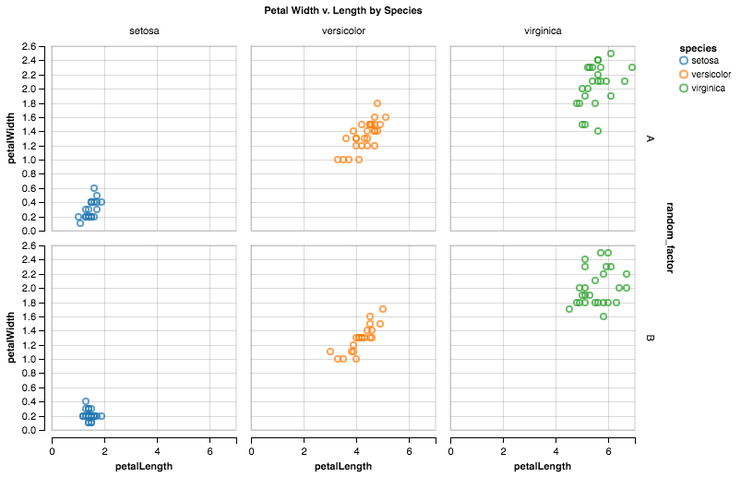
Just one more argument to the “encode” function than we had above!
Hopefully, the advantages of having faceting built into your visualization library’s framework are clear.

“编码”功能仅比我们上面提到的多一个！
希望将刻面内置到可视化库框架中的好处很明显。

ACT 2：分配和禁止 (ACT 2: DISTRIBUTIONS AND BARS)

场景4：您将如何可视化分布？ (Scene 4: How would you visualize distributions?)

MPL (confidence visibly shaken): Well, if we wanted a boxplot — do we want a boxplot? — I have a way of doing it. It’s stupid; you’d hate it. But I pass an array of arrays to my boxplot method, and this produces a boxplot for each subarray. You’ll need to manually label the x-ticks yourself.

MPL （明显动摇的信心）：好吧，如果我们想要一个箱线图—我们想要一个箱线图吗？ —我有办法做到。这很傻; 你会讨厌的。但是我将一个数组数组传递给boxplot方法，这为每个子数组生成一个boxplot。您需要自己手动标记X标记。

# MATPLOTLIB
fig, ax = plt.subplots(1, 1, figsize=(10, 10))
ax.boxplot([df[df.species == s]['petalWidth'].values
for s in df.species.unique()])
ax.set(xticklabels=df.species.unique(),
xlabel='Species',
ylabel='Petal Width',
title='Distribution of Petal Width by Species')

# MATPLOTLIB
fig, ax = plt.subplots(1, 1, figsize=(10, 10))
ax.boxplot([df[df.species == s]['petalWidth'].values
for s in df.species.unique()])
ax.set(xticklabels=df.species.unique(),
xlabel='Species',
ylabel='Petal Width',
title='Distribution of Petal Width by Species')

MPL: And if we wanted a histogram — do we want a histogram? — I have a method for that, too, which you can produce using either the for loop or group by methods from before.

MPL ：如果我们想要一个直方图-我们想要一个直方图吗？ —我也有一个方法，您可以使用for循环或以前的group by方法生成该方法。

P (looking uncharacteristically proud): Ha! Hahahaha! This is my moment! You all thought I was nothing but matplotlib’s patsy, and although I’ve so far been nothing but a wrapper around his plot method, I possess special functions for both boxplots and histograms — these make visualizing distributions a snap. You only need two things: (A) The column name by which you’d like to stratify; and (B) The column name for which you’d like distributions. These go to the “by” and “column” parameters, respectively, resulting in instant plots!

P （看上去很反常）：哈！哈哈哈哈！这是我的时刻！你们都以为我不过是matplotlib的小病，尽管到目前为止我只是他的plot方法的包装器，但我对boxplot 和直方图都拥有特殊的功能-这些使可视化分布变得轻而易举。您只需要两件事：（A）您想要分层的列名；（B）您想要分配的列名。它们分别进入“ by”和“ column”参数，从而产生即时绘图！

# PANDAS
fig, ax = plt.subplots(1, 1, figsize=(10, 10))
df.boxplot(column='petalWidth', by='species', ax=ax)

# PANDAS
fig, ax = plt.subplots(1, 1, figsize=(10, 10))
df.boxplot(column='petalWidth', by='species', ax=ax)

GG and ALT high five and congratulate P; shouts of “awesome!”, “way to be!”, “let’s go!” audible

GG和ALT高五并祝贺P；喊着“很棒！”，“要成为！”，“走吧！” 可听见的

SB (feigning enthusiasm): Wooooow. Greeeeat. Meanwhile, in my world, distributions are exceedingly important, so I maintain special methods for them. For example, my boxplot method needs an x argument, a y argument, and data, resulting in this:

SB （假装热情）：哇。真吃同时，在我的世界中，分发非常重要，因此我为它们维护特殊的方法。例如，我的boxplot方法需要一个x参数，ay参数和数据，结果是：

# SEABORN
fig, ax = plt.subplots(1, 1, figsize=(10, 10))
g = sns.boxplot('species', 'petalWidth', data=df, ax=ax)
g.set(title='Distribution of Petal Width by Species')

# SEABORN
fig, ax = plt.subplots(1, 1, figsize=(10, 10))
g = sns.boxplot('species', 'petalWidth', data=df, ax=ax)
g.set(title='Distribution of Petal Width by Species')

SB: Which, I mean, some people have told me is beautiful… but whatever. I also have a special distribution method named “distplot” that goes beyond histograms (looks at pandas haughtily). You can use it for histograms, KDEs, and rugplots — even plotting them simultaneously. For example, by combining this method with FacetGrid, I can produce a histo-rugplot for every species of iris:

SB ：我的意思是，有人告诉我这很漂亮……但随便。我还有一种称为“ distplot”的特殊分布方法，它超出了直方图（傲慢地看着熊猫）。您可以将其用于直方图，KDE和曲线图，甚至可以同时绘制它们。例如，通过将此方法与FacetGrid结合使用，我可以为每种虹膜种类生成一个组织图：

SB: But again… whatever.

SB ：但是，再说一次。

GG: THESE ARE BOTH JUST NEW GEOMS! GEOM_BOXPLOT FOR BOXPLOTS AND GEOM_HISTOGRAM FOR HISTOGRAMS! JUST SWAP THEM IN! (starts running around the dinner table)

GG ：这些都是全新的宝石！用于直方图的GEOM_BOXPLOT和用于直方图的GEOM_HISTOGRAM！只需将它们交换！（开始在餐桌旁走动）

# GGPY
g = ggplot(df, aes(x='species',
y='petalWidth',
fill='species')) +
geom_boxplot() +
ggtitle('Distribution of Petal Width by Species')
g

# GGPY
g = ggplot(df, aes(x='species',
y='petalWidth',
fill='species')) +
geom_boxplot() +
ggtitle('Distribution of Petal Width by Species')
g

ALT (looking steely-eyed and confident): I… I have a confession…

ALT （看上去像钢眼和自信）：我……我有一个坦白的人……

silence falls — GG stops running and lets plate fall to the floor

沉默落下-GG停止运行，让板坠落在地板上

ALT: (breathing deeply) I… I… I can’t do boxplots. Never really learned how, but I trust the JavaScript grammar out of which I grew has a good reason for this. I can make a mean histogram, though…

ALT ：（深呼吸）我……我……我不能做箱线图。从来没有真正学过如何做，但是我相信我所成长JavaScript语法有充分的理由。不过，我可以制作平均直方图。

# ALTAIR
c = Chart(df).mark_bar(opacity=.75).encode(
x=X('petalWidth', bin=Bin(maxbins=30)),
y='count(*)',
color=Color('species', scale=Scale(range=cp.as_hex()))
)
c

# ALTAIR
c = Chart(df).mark_bar(opacity=.75).encode(
x=X('petalWidth', bin=Bin(maxbins=30)),
y='count(*)',
color=Color('species', scale=Scale(range=cp.as_hex()))
)
c

ALT: The code may look weird at first glance, but don’t be alarmed. All we’re saying here is: “Hey, histograms are effectively bar charts.” Their x-axes correspond to bins, which we can define with my Bin class; meanwhile, their y-axes correspond to the number of items in the data set which fall into those bins, which we can explain using a SQL-esque “count(*)” as our argument for y.

ALT ：乍一看，代码可能看起来很怪异，但不要惊慌。我们在这里所说的是：“嘿，直方图实际上是条形图。” 它们的x轴对应于bin，我们可以使用Bin类来定义它们。同时，它们的y轴对应于数据集中属于这些bin的项目数，我们可以使用SQL式的“ count（*）”作为y的参数进行解释。

分析场景4 (Analyzing Scene 4)

In my work, I actually find pandas’ convenience functions very convenient; however, I’ll admit that there’s some cognitive overhead in remembering that pandas has implemented a “by” parameter for boxplots and histograms but not for lines.
I separate Act 1 from Act 2 for a few reasons, and a big one is this: Act 2 is when using matplotlib gets particularly hairy. Remembering a totally separate interface when you want a boxplot, for example, doesn’t work for me.
Speaking of Act 1 v. Act 2, a fun story: I actually came to Seaborn from matplotlib/pandas for its rich set of “proprietary” visualization functions (e.g., distplot, violin plots, regression plots, etc.). While I later learned to love FacetGrid, I maintain that it’s these Act 2 functions which are Seaborn’s killer app. They’ll keep me a Seaborn fan as long as I plot.
(Moreover, I need to note: Seaborn implements a number of awesome visualizations that lesser libraries ignore; if you’re in the market for one of these, then Seaborn is your only option.)
These examples are really when you begin to grok the power of ggpy’s geom system. Using mostly the same code (and more importantly, mostly the same thought process), we create a wildly different graph. We do this not by calling an entirely separate function, but by changing how our aesthetic mappings get presented to the viewer, i.e., by swapping out one geom for another.
Similarly, even in the world of Act 2, Altair’s API remains remarkably consistent. Even for what feels like a different operation, Altair’s API is simple, elegant, and expressive.

在工作中，我实际上发现熊猫的便利功能非常便利；但是，我要承认，记住熊猫已经为箱线图和直方图而不是线实现了“ by”参数，这会产生一些认知上的负担。
我出于某些原因将Act 1与Act 2分开，其中一个重要原因是：Act 2在使用matplotlib时显得特别毛茸茸。例如，当您想要箱线图时，记住一个完全独立的界面对我不起作用。
说到第一幕诉第二幕，一个有趣的故事：我实际上是从matplotlib / pandas来到Seaborn的，因为它具有丰富的“专有”可视化功能集（例如distplot，小提琴图，回归图等）。当我后来学会了爱FacetGrid时，我坚持认为这是Act 2的功能，它们是Seaborn的杀手级应用。只要我密谋，他们就会让我成为Seaborn粉丝。
（此外，我需要指出：Seaborn实现了一些很棒的可视化，而较少的库会忽略；如果您在其中的其中一种市场上，那么Seaborn是您唯一的选择。）
这些示例确实是在您开始了解ggpy的geom系统功能时。使用几乎相同的代码（更重要的是，几乎相同的思维过程），我们创建了完全不同的图。我们这样做不是通过调用一个完全独立的函数，而是通过更改我们的美学映射呈现给查看者的方式，即将一个几何替换为另一个。
同样，即使在《 Act 2》的世界中，Altair的API仍然保持着一致。即使感觉不同，Altair的API仍简单，优雅且富有表现力。

Data Aside

暂存数据

(In the final scene, we’ll be dealing with “titanic,” another famous tidy dataset [although again, we refer to it as “df” in our code]. Here’s a preview…)

（在最后一幕中，我们将处理另一个著名的整洁数据集“ titanic”（尽管在我们的代码中再次将其称为“ df”）。这是一个预览…）

		survived	幸存下来	pclass	p类	sex	性别	age	年龄	fare	票价	class	类
0	0	0	0	3	3	male	男	22.0	22.0	7.2500	7.2500	Third	第三
1	1个	1	1个	1	1个	female	女	38.0	38.0	71.2833	71.2833	First	第一
2	2	1	1个	3	3	female	女	26.0	26.0	7.9250	7.9250	Third	第三
3	3	1	1个	1	1个	female	女	35.0	35.0	53.1000	53.1000	First	第一
4	4	0	0	3	3	male	男	35.0	35.0	8.0500	8.0500	Third	第三

In this example, we’ll be interested in looking at the average fare paid by class and by whether or not somebody survived. Obviously, you could do this in pandas…

在此示例中，我们将关注按班级支付的平均票价以及是否有人幸免。显然，您可以在熊猫中做到这一点……

				fare	票价
survived	幸存下来	pclass	p类
0	0	1	1个	64.684008	64.684008
		2	2	19.412328	19.412328
		3	3	13.669364	13.669364
1	1个	1	1个	95.608029	95.608029
		2	2	22.055700	22.055700
		3	3	13.694887	13.694887

…but what fun is that? This is a post on visualization, so let’s do it in the form of a bar chart!)

…那是什么乐趣？这是关于可视化的文章，所以我们以条形图的形式来做！）

场景5：如何创建条形图？ (Scene 5: How would you create a bar chart?)

MPL (looking grim): No comment.

MPL （表情严峻）：无可奉告。

# MATPLOTLIB
died = dfg.loc[0, :]
survived = dfg.loc[1, :]
# more or less copied from matplotlib's own
# api example
fig, ax = plt.subplots(1, 1, figsize=(12.5, 7))
N = 3
ind = np.arange(N)  # the x locations for the groups
width = 0.35        # the width of the bars
rects1 = ax.bar(ind, died.fare, width, color='r')
rects2 = ax.bar(ind + width, survived.fare, width, color='y')
# add some text for labels, title and axes ticks
ax.set_ylabel('Fare')
ax.set_title('Fare by survival and class')
ax.set_xticks(ind + width)
ax.set_xticklabels(('First', 'Second', 'Third'))
ax.legend((rects1[0], rects2[0]), ('Died', 'Survived'))
def autolabel(rects):
# attach some text labels
for rect in rects:
height = rect.get_height()
ax.text(rect.get_x() + rect.get_width()/2., 1.05*height,
'%d' % int(height),
ha='center', va='bottom')
ax.set_ylim(0, 110)
autolabel(rects1)
autolabel(rects2)
plt.show()

# MATPLOTLIB
died = dfg.loc[0, :]
survived = dfg.loc[1, :]
# more or less copied from matplotlib's own
# api example
fig, ax = plt.subplots(1, 1, figsize=(12.5, 7))
N = 3
ind = np.arange(N)  # the x locations for the groups
width = 0.35        # the width of the bars
rects1 = ax.bar(ind, died.fare, width, color='r')
rects2 = ax.bar(ind + width, survived.fare, width, color='y')
# add some text for labels, title and axes ticks
ax.set_ylabel('Fare')
ax.set_title('Fare by survival and class')
ax.set_xticks(ind + width)
ax.set_xticklabels(('First', 'Second', 'Third'))
ax.legend((rects1[0], rects2[0]), ('Died', 'Survived'))
def autolabel(rects):
# attach some text labels
for rect in rects:
height = rect.get_height()
ax.text(rect.get_x() + rect.get_width()/2., 1.05*height,
'%d' % int(height),
ha='center', va='bottom')
ax.set_ylim(0, 110)
autolabel(rects1)
autolabel(rects2)
plt.show()

everyone else shakes their head

其他人都摇头

P: I need to do some data manipulation first — namely, a group by and a pivot — but once I do, I have a really cool bar chart method — much simpler than that mess above! Wow, I’m feeling so much more confident — who knew all I had to was put someone else down!?⁵

警：我需要先做一些数据操作，即分组和枢轴操作，但是一旦完成，我就会有一个非常酷的条形图方法，比上面的混乱要简单得多！哇，我感到更加自信-谁知道我要把别人压倒！！ ⁵

SB: Again, I happen to think tasks such as this are extremely important. As such, I implement a special function named “factorplot” to help out:

SB ：同样，我碰巧认为这样的任务非常重要。因此，我实现了一个名为“ factorplot”的特殊功能来帮助您：

# SEABORN
g = sns.factorplot(x='class', y='fare', hue='survived',
data=df, kind='bar',
order=['First', 'Second', 'Third'],
size=7.5, aspect=1.5)
g.ax.set_title('Fare by survival and class')

# SEABORN
g = sns.factorplot(x='class', y='fare', hue='survived',
data=df, kind='bar',
order=['First', 'Second', 'Third'],
size=7.5, aspect=1.5)
g.ax.set_title('Fare by survival and class')

SB: As ever, you pass in your un-manipulated data frame. Next, you explain what you would like to group by — in this case, it’s “class” and “survived,” so these become our “x” and “hue” arguments. Next, you explain what numeric field you would like summaries for — in this case, it’s “fare,” so this becomes our “y” argument. The default summary statistic is mean, but factorplot possesses a parameter named “estimator,” where you can specify any function you want, e.g., sum, standard deviation, median, etc. The function you choose will determine the height of each bar.

SB ：和往常一样，您传入未经处理的数据框。接下来，您要解释要分组的内容-在这种情况下，它是“类”和“生存”的，因此它们成为我们的“ x”和“色相”参数。接下来，说明您想要摘要的数字字段-在这种情况下为“票价”，因此这成为我们的“ y”参数。默认的摘要统计量是平均值，但是factorplot具有一个名为“估计量”的参数，您可以在其中指定所需的任何函数，例如求和，标准差，中位数等。您选择的函数将确定每个条形的高度。

Of course, there are many ways to visualize this information, only one of which is a bar. As such, I also have a “kind” parameter where you can specify different visualizations.

当然，有很多方法可以可视化此信息，其中只有一种是条形图。因此，我还有一个“种类”参数，您可以在其中指定不同的可视化效果。

Finally, some of us still care about statistical certainty, so by default, I bootstrap you some error bars so you can see if the differences in average fair between classes and survivorship are meaningful.

最后，我们中的某些人仍然关心统计的确定性，因此默认情况下，我会引导您一些误差线，以便您可以查看类和生存率之间的平均公平差异是否有意义。

(under her breath) Would like to see any of you top that…

（在她的呼吸下）想看到你们中的任何一个……

ggplot2 pulls up in his Lamborghini and walks through the door

ggplot2拉起他的兰博基尼，走进门

ggplot2: Hey, have y’all see–

ggplot2 ：嘿，你们都看到了吗？

GG: HEY BRO.

GG ：嘿，兄弟。

GG2: Hey, little man. We gotta go.

GG2 ：嘿，小矮人。我们要走了。

GG: Wait, one sec — I gotta make this bar plot real quick, but I’m having a hard time. How would you do it?

GG ：等等，一秒钟-我得快速绘制出这个条形图，但是我很难过。你会怎么做？

GG2 (reading instructions): Ah, like this:

GG2 （阅读说明）：啊，像这样：

GG2: See? You define your aesthetic mappings like we always talk about, but you need to turn your “y” mapping into average fare. To do so, I get my pal “stat_summary_bin” to do that for me by passing in “mean” to his “fun.y” parameter.

GG2 ：看到了吗？您可以像我们经常谈论的那样定义美学映射，但是您需要将“ y”映射转换为平均票价。为此，我将“ mean”传递给他的“ fun.y”参数，让我的朋友“ stat_summary_bin”为我完成此操作。

GG (eyes wide in amazement): Oh, whoa… I don’t think I have stat_summary yet. I guess — pandas, could you help me out?

GG （惊讶地睁大了眼睛）：哦，哇……我认为我还没有stat_summary。我想-熊猫，你能帮帮我吗？

P: Uh, sure.

警：嗯，当然。

GG: Weeeee!

GG ：We！

# GGPY
g = ggplot(df.groupby(['class', 'survived']).
agg({'fare': 'mean'}).
reset_index(), aes(x='class',
fill='factor(survived)',
weight='fare',
y='fare')) +
geom_bar() +
ylab('Avg. Fare') +
xlab('Class') +
ggtitle('Fare by survival and class')
g

# GGPY
g = ggplot(df.groupby(['class', 'survived']).
agg({'fare': 'mean'}).
reset_index(), aes(x='class',
fill='factor(survived)',
weight='fare',
y='fare')) +
geom_bar() +
ylab('Avg. Fare') +
xlab('Class') +
ggtitle('Fare by survival and class')
g

GG2: Huh, not exactly grammar of graphics-approved, but I guess so long as Hadley doesn’t find out it seems to work fine… In particular, you shouldn’t have to summarize your data in advance of your visualization. I’m also confused by what “weight” means in this context…

GG2 ：呵呵，不是完全经过图形批准的语法，但是我想只要Hadley没发现它看起来可以正常工作……尤其是，您不必在可视化之前总结数据。在这种情况下，“重量”的含义也让我感到困惑。

GG: Well, by default, my bar geom seems to default to simple counts, so without a “weight,” all the bars would have had a height of one.

GG ：好吧，默认情况下，我的条形图似乎默认为简单计数，因此，如果没有“重量”，则所有条形的高度都将为一。

GG2: Ah, I see… Let’s talk about that later.

GG2 ：啊，我明白了……让我们稍后再谈。

GG and GG2 say their goodbyes and leave the dinner party

GG和GG2告别，离开晚宴

ALT: Ah, now this is my bread-and-butter. It’s really simple.

阿尔特 ：啊，现在这是我的面包。真的很简单。

ALT: I’m hoping all the arguments are intuitive by this point: I want to plot mean fare by survivorship — faceted by class. This directly translates into “survived” as the x argument; “mean(fare)” as the y argument; and “class” as the column argument. (I specify the color argument for some pizazz.)

ALT ：到目前为止，我希望所有论点都是直观的：我想按生存率（按班级划分）绘制平均票价。这直接转换为“生存”作为x参数； “平均（票价）”作为y参数；并以“ class”作为列参数。（我为一些爵士乐指定了color参数。）

That said, a couple of new things are happening here. Notice how I append “:N” to the “survived” string in the x and color arguments. This is a note to myself which says, “This is a nominal variable.” I need to put this here because survived looks like a quantitative variable, and a quantitative variable would lead to a slightly uglier visualization of this plot. Don’t be alarmed: this has been happening the whole time — just implicitly. For example, in the time series plots above, if I hadn’t known “dt” was a temporal variable I would have assumed they were nominal variables, which… would have been awkward (at least until I appended “:T” to clear things up.

就是说，这里发生了几件事。注意如何在x和color参数中将“：N”附加到“幸存”字符串中。这是给自己的便条，上面写着“这是一个名义变量”。我需要将其放在此处，因为幸存的对象看起来像是一个定量变量，而定量变量将导致该图的可视化效果稍差一些。不要惊慌：这一直在发生-只是在隐式地发生。例如，在上面的时间序列图中，如果我不知道“ dt”是一个时间变量，我会假定它们是名义变量，这……会很尴尬（至少直到我附加“：T”以清除事情了。

Separately, I invoke my configure_facet_cell protocol to make my three subplots look more unified.

另外，我调用了configure_facet_cell协议，使我的三个子图看起来更加统一。

分析场景5 (Analyzing Scene 5)

Don’t overthink this one: I’m never making a bar chart in matplotlib again, and to be clear, it’s nothing personal! The fact is: unlike the other libraries, matplotlib doesn’t have the luxury of making any assumptions about the data it receives. Occasionally, this means you’ll have pedantically imperative code.
(Of course, it’s this same data agnosticism that allows matplotlib to be the foundation upon which Python visualization is built.)
Conversely, whenever I need summary statistics and error bars, I will always and forever turn to Seaborn.
(It’s potentially unfair I chose an example that seems tailor-made to one of Seaborn’s functions, but it comes up a lot in my work, and hey, I’m writing the blog post here.)
I don’t find either the pandas approach or the ggpy approach particularly offensive.
However, in the pandas case, knowing you must group by and pivot — all in service of a simple bar chart — seems a bit silly.
Similarly, I do think this is the main hole I’ve found in yhat’s ggpy — having a “stat_summary” equivalent would go a long way toward making this thing wonderfully full-featured.
Meanwhile, Altair continues to impress! I was struck by how intuitive the code was for this example. Even if you’d never seen Altair before, I imagine someone could intuit what was happening. It’s this type of 1:1:1 mapping between thinking, code, and visualization that is my favorite thing about the library.

不要想太多了：我再也不会在matplotlib中制作条形图了，并且要明确的是，这并不是什么私人的！事实是：与其他库不同，matplotlib没有奢侈地对其接收的数据进行任何假设。有时，这意味着您将拥有脚踏式命令性代码。
（当然，正是这种相同的数据不可知论使matplotlib成为构建Python可视化的基础。）
相反，每当我需要汇总统计信息和错误栏时，我将永远永远求助于Seaborn。
（我选择了一个似乎是针对Seaborn的功能之一量身定制的示例，这可能是不公平的，但是这在我的工作中起了很大作用，嘿，我在这里写博客。）
我认为熊猫方法或ggpy方法都不是特别令人反感的方法。
但是，在大熊猫的情况下，知道您必须分组并进行枢纽操作（所有工作都只是简单的条形图）似乎有点愚蠢。
同样，我确实认为这是我在yhat的ggpy中发现的主要漏洞-具有“ stat_summary”等效项将大大有助于使此功能功能完善。
同时，Altair继续给您留下深刻印象！我对这个示例的代码如此直观感到震惊。即使您以前从未见过Altair，我也可以想象有人可以了解正在发生的事情。我在库中最喜欢的就是这种思维，代码和可视化之间的1：1：1映射类型。

最后的想法 (Final Thoughts)

You know, sometimes I think it’s important to just be grateful: we have a ton of great visualization options, and I enjoyed digging into all of them!

您知道，有时候我觉得感恩是很重要的：我们有大量出色的可视化选项，我喜欢深入研究所有这些选项！

(Yes, this is a cop-out.)

（是的，这是应对措施。）

Although I was a bit hard on matplotlib, it was all in good fun (every play needs comedic relief). Not only is matplotlib the foundation upon which pandas plotting, Seaborn, and ggpy are built, but the fine-grained control he gives you is essential. I didn’t touch on this, but in almost every non-Altair example, I used matplotlib to customize our final graph. But — and this is a big “but” — matplotlib is purely imperative, and specifying your visualization in exacting detail can get tedious (see: bar chart).

尽管我在使用matplotlib时有些困难，但一切都很好玩（每个游戏都需要喜剧缓解）。 matplotlib不仅是构建大熊猫绘图，Seaborn和ggpy的基础，而且他给您的细粒度控制至关重要。我没有涉及这个问题，但是在几乎每个非Altair的示例中，我都使用matplotlib自定义了最终图形。但是-这是一个很大的“但是”-matplotlib是绝对必要的，并且详细指定可视化内容可能会变得乏味（请参阅：条形图）。

Indeed, the upshot here is probably: “Judging matplotlib on the basis of its statistical visualization capabilities is kind of unfair, you big meanie. You’re comparing one of its use cases to the other libraries’ primary use case. These approaches obviously need to work together. You can use your preferred convenience/declarative layer — pandas, Seaborn, ggpy, or one day Altair (see below) — for the basics. Then you can use matplotlib for the non-basics. When you run up against the limitations of what these other libraries can do, you’ll be happy to have the limitless power of matplotlib at your side, you ungrateful aesthetic amateur.”

确实，这里的结果可能是：“根据其统计可视化功能判断matplotlib有点不公平，您是个卑鄙的人。您正在将其用例之一与其他库的主要用例进行比较。这些方法显然需要协同工作。您可以使用首选的便利/声明层-大熊猫，Seaborn，ggpy或一日Altair（请参阅下文）作为基础。然后，您可以将matplotlib用于非基础知识。当您遇到其他这些库所不能提供的限制时，您会很高兴拥有matplotlib的无限功能，这是您忘恩负义的业余爱好者。”

To which I’d say: yes! That seems quite sensible, Disembodied Voice… although just saying that wouldn’t make for much of a blog post.

我要说的是：是的！这似乎很明智，“无形的声音”……尽管只是说那并不能构成很多博客文章。

Plus… I could do without the name-calling