FAU深度学习讲义 (FAU Lecture Notes in Deep Learning)

These are the lecture notes for FAU’s YouTube Lecture “Deep Learning”. This is a full transcript of the lecture video & matching slides. We hope, you enjoy this as much as the videos. Of course, this transcript was created with deep learning techniques largely automatically and only minor manual modifications were performed. If you spot mistakes, please let us know!

这些是FAU YouTube讲座“ 深度学习 ”的 讲义 。 这是演讲视频和匹配幻灯片的完整记录。 我们希望您喜欢这些视频。 当然，此成绩单是使用深度学习技术自动创建的，并且仅进行了较小的手动修改。 如果发现错误，请告诉我们！

导航 (Navigation)

Previous Lecture / Watch this Video / Top Level / Next Lecture

上一个讲座 / 观看此视频 / 顶级 / 下一个讲座

Welcome, everybody to our next video on deep learning! So, today we want to talk about again feed-forward networks. In the fourth part, the main focus will be on the layer abstraction. Of course, we talked about those neurons and individual nodes but this grows really complex for larger networks. So we want to introduce this layering concept also in our computation of the gradients. This is really useful because we can then talk directly about gradients on entire layers and don’t need to go towards all of the different nodes.

欢迎大家观看我们的下一个有关深度学习的视频！ 因此，今天我们要再次讨论前馈网络。 在第四部分中，主要重点将放在层抽象上。 当然，我们讨论了那些神经元和单个节点，但是对于大型网络而言，这变得非常复杂。 因此，我们也想在梯度计算中引入这种分层概念。 这真的很有用，因为我们可以直接讨论整个图层上的渐变，而无需遍历所有不同的节点。

So, how do we express this? Let’s recall what our single neuron is doing. The single neuron is computing essentially an inner product of its weights. By the way, we are skipping over this bias notation. So, we are expanding this vector by one additional element. This allows us to describe the bias also and the inner product as shown on the slide here. This is really nice because then you can see that the output y hat is just an inner product.

那么，我们该如何表达呢？ 让我们回想一下我们的单个神经元在做什么。 单个神经元实际上是在计算其权重的内积。 顺便说一下，我们跳过了这个偏见符号。 因此，我们将这个向量扩展一个额外的元素。 这使我们也可以描述偏差和此处幻灯片所示的内积。 这非常好，因为您可以看到输出y只是一个内部产品。

Now think about the case that we have M neurons which means that we get some y hat index m. All of them are inner products. So, if you bring this into a vector notation, you can see that the vector y hat is nothing else than a matrix multiplication of x with this matrix W. You see that a fully connected layer is nothing else than matrix multiplication. So, we can essentially represent arbitrary connections and topologies using this fully connected layer. Then, we also apply a pointwise non-linearity such that we get the nonlinear effect. The nice thing about matrix notation is of course that we can describe now the entire layer derivatives using matrix calculus.

现在考虑一下我们有M个神经元的情况，这意味着我们得到了y指数m 。 它们都是内部产品。 因此，如果将其引入向量符号中，则可以看到向量y hat就是x与该矩阵W的矩阵乘法。 您会看到一个完全连接的层就是矩阵乘法。 因此，我们基本上可以使用此完全连接的层表示任意连接和拓扑。 然后，我们还应用逐点非线性，从而获得非线性效应。 关于矩阵表示法的好处当然是我们现在可以使用矩阵演算来描述整个层的导数。

So, our fully connected layer would then get the following configuration: Three elements for the input and then weights for every neuron. Let’s say you have two neurons, then we get these weight vectors. We multiply the two with x. In the forward pass, we have determined this y hat for the entire module using a matrix. If you want to compute the gradients, then we need exactly two partial derivatives. These are the same as we already mentioned: We need the derivative with respect to the weights. This is going to be the partial derivative with respect to W and the partial derivatives with respect to x for the backpropagation to pass it on to the next module.

因此，我们的全连接层将获得以下配置：输入三个元素，然后每个神经元加权。 假设您有两个神经元，那么我们得到了这些权重向量。 我们将两者乘以x 。 在正向通，我们已经确定了使用矩阵整个模块此ÿ帽子。 如果要计算梯度，则我们需要两个偏导数。 这些与我们已经提到的相同：我们需要权重的导数。 对于反向传播，这将是相对于W的偏导数和相对于x的偏导数，以将其传递到下一个模块。

So how do we compute this? Well, we have the layer that is y hat equals to W x. So there’s a matrix multiplication in the forward pass. Then, we need the derivative with respect to the weights. Now you can see that what we essentially need to do is we need a matrix derivative here. The derivative of y hat with respect to W is going to be simply xᵀ. So, if we have the loss that comes into our module, the update to our weights is gonna be this loss vector multiplied with xᵀ. So, we have some loss vector and xᵀ which essentially means that you have an outer product. One is a column vector and the other one is a row vector because of the transpose. So, if you multiply the two, you will end up with a matrix. The above partial derivative with respect to W will always result in a matrix. Then if you look at the bottom row, you need the partial derivative of y hat with respect to x. Also something you can find in the matrix cookbook, by the way. It is very very useful. You find all kinds of matrix derivatives in this one. So if you do that, you can see for the above equation, the partial with respect to x is going to be Wᵀ. Now, you have Wᵀ multiplied again by some loss vector. This loss vector times a matrix is going to be a vector again. This is the vector that you will pass on in the backpropagation process towards the next higher layer.

那么我们如何计算呢？ 好吧，我们拥有的层y等于W x 。 因此，在前向通过中存在矩阵乘法。 然后，我们需要权重的导数。 现在您可以看到，我们本质上需要做的就是在这里需要矩阵导数。 y hat对W的导数将只是x x 。 因此，如果我们有一个进入我们的模块损失，更新我们的权重是要成为这个丢失向量乘以Xᵀ。 所以，我们有一些丢失向量和Xᵀ这实际上是说你有一个外部的产品。 由于转置，一个是列向量，另一个是行向量。 因此，如果将两者相乘，将得到一个矩阵。 上述关于W的偏导数将始终生成矩阵。 然后，如果查看底行，则需要y hat相对于x的偏导数。 顺便说一句，您也可以在矩阵食谱中找到一些东西。 这是非常非常有用的。 您可以在这一本书中找到各种矩阵导数。 所以，如果你这样做，你可以看到上面的方程，部分相对于X向为Wᵀ。 现在，您将W again再次乘以某个损失矢量。 该损失向量乘以矩阵将再次成为向量。 这是您将在反向传播过程中传递给下一个更高层的向量。

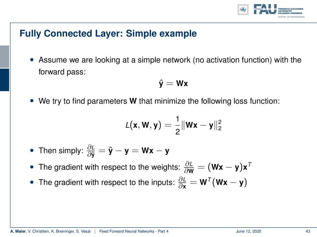
Okay so let’s look into some example. We have a simple example first and then a multi-layer example next. So, the simple example is going to be the same network as we had it already. So this was network without any non-linearity W x. Now, we need some loss function. Here, we don’t take cross-entropy, but we take the L2 loss which is a common vector norm. What it does is simply take the output of the network subtract and the desired output and compute the L2 norm. This means that we element-wise square the different vector values and sum all of them up. In the end, we would have to take a square root, but we want to omit this. So, we take it to the power of two. When we now compute the derivatives of this L2-norm to the power of 2, of course, we have a factor of two showing up. This will be canceled out by this factor 1 over 2 in the beginning. By the way, this is a regression loss and also has statistical relations. We will talk about this when we talk about loss functions in more detail. The nice thing with L2 loss is that that you also find its matrix derivatives the matrix cookbook. We now compute the partial derivative of L with respect to y hat. This will give us then Wx — y and we can continue and compute the update for our weights. So the update for the weights is what we compute using the loss function’s derivative. The derivative of the loss function with respect to the input was Wx — y times xᵀ. This will give us an update for the matrix weight. The other derivative that we want to compute is the partial derivative of the loss with respect to x. So, this is going to be — as we’ve seen on the previous slide — Wᵀ times the vector that comes from the loss function: Wx — y, as we determined in the third row of the slide.

好吧，让我们来看一些例子。 我们首先有一个简单的示例，然后是一个多层示例。 因此，简单的示例将是与我们已经拥有的相同的网络。 因此，这是一个没有任何非线性W x的网络 。 现在，我们需要一些损失函数。 在这里，我们不采用交叉熵，而是采用L2损失，这是一种常见的向量范数。 它所做的只是将网络的输出与所需的输出相减，然后计算L2范数。 这意味着我们逐个元素地对不同的矢量值求平方并将它们全部求和。 最后，我们必须取平方根，但是我们想忽略这一点。 因此，我们将其取二。 现在，当我们现在将此L2范数的导数计算为2的幂时，显示出来的系数就是2。 开始时，将通过这个因子2抵消1。 顺便说一下，这是一个回归损失，也有统计关系。 当我们更详细地讨论损失函数时，我们将讨论这一点。 L2损失的好处是您还可以找到矩阵食谱的矩阵导数。 现在我们计算关于y hat的L的偏导数。 这将给我们Wx - y ，我们可以继续计算权重的更新。 因此，权重的更新是我们使用损失函数的导数计算得出的。 相对于输入端的损耗函数的导数是蜡质 - y倍的xᵀ。 这将为我们提供矩阵权重的更新。 我们要计算的另一个导数是损耗相对于x的偏导数。 所以，这将是-正如我们看到的上一张幻灯片- 含 ᵀ倍来自于损失函数的向量：WX - Y，因为我们在幻灯片的第三行中确定。

Ok so let’s add some layers and change our estimator into three nested functions. Here, we have some linear matrices. So, this is an academic example: you could see that by multiplying W₁, W₂, and W₃ with each other, they would simply collapse into a single matrix. Still, I find this example useful because it shows you what actually happens in the computation of the backpropagation process and why those specific steps are really useful. So, again we take the L2 loss function. Here, we have our three matrices inside.

好的，让我们添加一些图层并将估算器更改为三个嵌套函数。 在这里，我们有一些线性矩阵。 因此，这是一个学术示例：您可以看到，通过将W ， W 2和W彼此相乘，它们将简单地折叠成一个矩阵。 不过，我发现此示例仍然有用，因为它向您展示了反向传播过程的计算中实际发生的情况以及为什么这些特定步骤真正有用。 因此，我们再次采用L2损失函数。 在这里，我们有我们的三个矩阵。

Next, we have to go ahead and compute derivatives. Now for the derivatives, we start with Layer 3, the most outer layer. So, you see that we now compute the partial derivative of the loss function with respect to W₃. First, the chain rule. Then, we have to compute the partial derivative of the loss function with respect to f₃(x) hat with respect to W₃. The partial derivative of the loss function again is simply the inner part of the L2 norm. So is this W₃ W₂ W₁ x — y. The partial derivative of the net is gonna be (W₂ W₁ x)ᵀ, as we’ve seen on the previous slide. Note that I’m indicating the affinity of the matrix operator using a dot. For matrices, it makes a difference whether you multiply them from the left or from the right. Both multiplication directions are different. Hence, I’m indicating that you have to compute this product from the right-hand side. Now let’s do that and we end up with the final update for W₃ that is simply computed from those two expressions.

接下来，我们必须继续计算导数。 现在，对于衍生工具，我们从最外层的第3层开始。 因此，您看到我们现在针对W compute计算损失函数的偏导数。 首先，连锁规则。 然后，我们必须针对f W ( x )hat相对于W₃计算损失函数的偏导数。 损失函数的偏导数再次只是L2范数的内部。 因此，这是W 3 w ^ w ^₂₁X - 年 。 净的偏导数是会是(W₂W¯¯₁x)的 ᵀ，正如我们所看到的前一幻灯片。 请注意，我使用点指示矩阵运算符的相似性。 对于矩阵，从左还是从右相乘会有所不同。 两个乘法方向都不相同。 因此，我表示您必须从右侧计算此乘积。 现在我们来做，最后得到W₃的最终更新，该更新仅从这两个表达式计算得出。

Now, the partial derivative with respect to W₂ is a bit more complicated because we have to apply the chain rule twice. So, again we have to compute the partial derivative of the loss function with respect to f₃(x) hat. Then, we need the partial derivative of f₃(x) hat with respect to W₂ which means we have to apply the chain rule again. So we have to expand the partial derivative of f₃(x) hat with respect to f₂(x) hat and then the partial derivative of f₂(x) hat with respect to W₂. This doesn’t change much. The Loss term is the same as we used before. Now, if we compute the partial derivative of f₃(x) hat with respect to f₂(x) hat — remember f₂(x) = W₂ W₁ x — it’s gonna be W₃ᵀ and we have to multiply it from the left-hand side. Then, we go ahead and compute the partial derivative of f₂(x) hat with respect to W₂. You remain with (W₂ W₁ x)ᵀ. So, the final matrix derivative is going to be the product of the three terms. We can repeat this for the last layer, but now we have to apply the chain rule again. We see already two parts that we pre-computed, but we have to apply it again. So here we then get the partial derivative of f₂(x) hat with respect to f₁(x) hat and a partial derivative of f₁(x) hat with respect to W₁ which then yields two terms that we used before. The partial derivative of f₂(x) hat with respect to f₁(x) hat is W₁ x, is going to be W₂ᵀ. Then, we still have to compute the partial derivative of f₁(x) with respect to W₁. This is going to be xᵀ. So, we end up with the product of four terms for this partial derivative.

现在，关于W 2的偏导数要复杂一些，因为我们必须两次应用链式规则。 因此，我们再次必须针对f₃( x )hat计算损失函数的偏导数。 然后，我们需要相对于W 2的f with( x )hat的偏导数，这意味着我们必须再次应用链式规则。 因此，我们必须扩大f₃( x )hat相对于f 2( x )hat的偏导数，然后扩大f 2( x )hat关于W 2的偏导数。 这变化不大。 损失项与我们之前使用的相同。 现在，如果我们计算F 3(x)的帽子的偏导数相对于F 2(x)的帽子-记为f 2(x)= W₂W¯¯₁X -它会为W₃ᵀ，我们必须从左边乘以手。 然后，我们继续计算f 2( x )hat相对于W 2的偏导数。 你留在(W₂W¯¯₁X)ᵀ。 因此，最终的矩阵导数将是这三个项的乘积。 我们可以在最后一层重复此操作，但是现在我们必须再次应用链式规则。 我们已经看到我们已经预先计算了两个部分，但是我们必须再次应用它。 所以在这里我们再拿到F 2(x)的帽子的偏导数相对于为f1(x)的帽子，并为f1(x)的帽子对w₁然后产生了两个方面，我们之前使用的偏导数。 F 2(x)的帽子相对于为f1(x)的帽子的偏导数为W₁X，是要为W₂ᵀ。 然后，我们还是要计算为f 1(X)的偏导数与W₁。 这将是xᵀ 。 因此，我们最终得到了该偏导数的四个项的乘积。

Now, you can see if we do the backpropagation algorithm, we end up in a very similar way of processing. So first, we compute the forward path through our entire network and evaluate the loss function. Then, we can look at the different partial derivatives, and depending on where I want to go, I have to compute the respective partials. For the update of the last layer, I have to compute the partial derivative of the loss function and multiply it with the partial derivative of the last layer with respect to the weights. Now, if I go the second last layer, I have to compute the partial derivative with respect to the loss function, the partial derivative of the last layer from respect to the inputs, and the partial derivative of the second last layer with respect to the weights to get the update. If I want to go to the first layer, I have to compute all the respective backpropagation steps for the entire layers until I end up with the respective update on the very first layer. You can see that we can pre-compute a lot of those values and reuse them which allows us to implement backpropagation very efficiently.

现在，您可以看到是否执行反向传播算法，最终以非常类似的方式进行处理。 因此，首先，我们计算整个网络的前向路径并评估损耗函数。 然后，我们可以查看不同的偏导数，并且根据我要去的地方，我必须计算相应的偏导数。 为了更新最后一层，我必须计算损失函数的偏导数，并将其与权重相关的最后一层的偏导数相乘。 现在，如果我走到倒数第二层，我必须计算相对于损失函数的偏导数，相对于输入的最后一层的偏导数以及相对于输入的倒数第二层的偏导数。权重以获取更新。 如果要转到第一层，则必须计算整个层的所有相应反向传播步骤，直到最终在第一层得到相应的更新。 您会看到我们可以预先计算很多这些值并重用它们，这使我们可以非常有效地实施反向传播。

Let’s summarize what we’ve seen so far. We’ve seen that we can combine the softmax activation function with the cross-entropy loss. Then, we can very naturally work with multi-class problems. We used gradient descent as the default choice for training network and we can achieve local minima using the strategy. We can, of course, compute gradients only numerically by finite differences and this is very useful for checking your implementations. This is something you will definitely need in the exercises! Then, we used the backpropagation algorithm to compute the gradients very efficiently. In order to be able to update the weights of the fully connected layers, we’ve seen that they can be abstracted as a complete layer. Hence, we can also compute layer-wise derivatives. So, it’s not required to compute everything on a node level, but you can really go into layer abstraction. You also saw that matrix calculus turns out to be very useful.

让我们总结一下到目前为止所看到的。 我们已经看到，我们可以将softmax激活函数与交叉熵损失结合起来。 然后，我们很自然地可以解决多类问题。 我们使用梯度下降作为训练网络的默认选择，并且可以使用该策略实现局部最小值。 当然，我们只能通过有限差分以数值方式计算梯度，这对于检查您的实现非常有用。 这是练习中肯定需要的东西！ 然后，我们使用反向传播算法非常有效地计算了梯度。 为了能够更新完全连接的层的权重，我们已经看到它们可以抽象为一个完整的层。 因此，我们还可以计算逐层导数。 因此，不需要在节点级别上计算所有内容，但是您确实可以进行层抽象。 您还看到了矩阵演算非常有用。

What happens next time in deep learning? Well, we will see that right now, we have only a limited number of loss functions. So, we will see problem adapted loss functions for regression and classification. The very simple optimization that we talked about right now with a single η is probably not the right way to go. So, there are much better optimization programs. They can be adapted to the needs of every single parameter. Then we’ll also see an argument why neural networks shouldn’t perform that well and some recent insights why they actually do perform quite well.

下次深度学习会发生什么？ 好吧，我们现在将看到，我们只有有限数量的损失函数。 因此，我们将看到适用于问题的损失函数，用于回归和分类。 我们现在仅用一个η讨论的非常简单的优化可能不是正确的方法。 因此，有更好的优化程序。 它们可以适应每个单个参数的需求。 然后，我们还将看到一个论点，为什么神经网络的性能不能这么好，以及一些最近的见解，为什么它们实际上确实表现得很好。

I also have a couple of comprehensive questions. So you should definitely be able to name different loss functions for multi-class classification. One-hot encoding is something everybody needs to know if you want to take the oral exam with me. You will have to be able to describe this. Then, of course, something I probably won’t ask in the exam but something that will be very useful for your daily routine is that you work with finite differences and use them for implementation checks. You have to be able to describe the backpropagation algorithm and to be honest, I think this — although it’s academic — but this multi-layer way abstraction way of describing backpropagation algorithm is really useful. It’s also very nice if you want to explain the backpropagation in an exam situation. What else do you have to be able to describe? The problem with exploding and vanishing gradients: What happens if you choose your η too high or too low? What’s a lost curve and how does it change over the iterations? Take a look at those graphs. They are really relevant and they also help you understand what’s going wrong in your training process. So you need to be aware of those and also it should be clear to you by now why the sign function is a bad choice for an activation function. We have plenty of references below this post. So, I hope you still had fun with those videos. Please continue watching and see you in the next video!

我也有几个全面的问题。 因此，您绝对应该能够为多类分类命名不同的损失函数。 如果您想和我一起参加口试，那么每个人都需要知道一键编码。 您将必须能够描述这一点。 然后，当然，我可能不会在考试中问到一些问题，但是对您的日常工作非常有用的一件事是您使用有限的差异并将其用于实现检查。 您必须能够描述反向传播算法，并且说实话，我认为这虽然是学术上的，但是这种描述反向传播算法的多层方式抽象方法确实很有用。 如果您想解释考试情况下的反向传播，也非常好。 您还必须描述什么？ 梯度爆炸和消失的问题：如果您选择的η太高或太低怎么办？ 什么是丢失曲线，它在迭代过程中如何变化？ 看看那些图。 它们确实相关，并且还可以帮助您了解培训过程中出了什么问题。 因此，您需要意识到这些，并且现在您应该已经明白为什么符号功能对于激活功能是错误的选择。 我们在这篇文章下面有很多参考。 因此，我希望您仍然喜欢那些视频。 请继续观看并在下一个视频中见！

If you liked this post, you can find more essays here, more educational material on Machine Learning here, or have a look at our Deep Learning Lecture. I would also appreciate a clap or a follow on YouTube, Twitter, Facebook, or LinkedIn in case you want to be informed about more essays, videos, and research in the future. This article is released under the Creative Commons 4.0 Attribution License and can be reprinted and modified if referenced.

如果你喜欢这篇文章，你可以找到这里更多的文章 ，更多的教育材料，机器学习在这里 ，或看看我们的深入 学习 讲座 。 如果您想在以后了解更多文章，视频和研究信息，也欢迎在YouTube ， Twitter ， Facebook或LinkedIn上进行拍手或追随。 本文是根据知识共享4.0署名许可发布的 ，如果引用，可以重新打印和修改。