In Death and Life of Great American Cities, the great Jane Jacobs lays out four essential characteristics of a great neighborhood:

在《美国大城市的死亡与生活》中 ，伟大的简·雅各布斯阐述了一个大社区的四个基本特征：

• Density密度
• A mix of uses多种用途
• A mix of building ages, types and conditions混合建筑年龄，类型和条件
• A street network of short, connected blocks短而相连的街区的街道网络

Of course, she goes into much greater detail on all of these, but I’m not going to get into all the eyes-on-the-street level stuff. Instead, I’m going to find neighborhoods with the right “bones” to build great urbanism onto. The caveat to this, as with most geospatial planning tools, is that it is not to be blindly trusted. There are a lot of details that need on the ground attention.

当然，她会在所有这些方面进行更详细的介绍，但我不会涉及所有在街头关注的内容。 取而代之的是，我将寻找具有正确“骨骼”的街区，以在其上建立伟大的城市主义。 与大多数地理空间规划工具一样，对此的警告是，不要盲目地信任它。 有很多需要地面关注的细节。

On to the data.

关于数据。

工具类 (Tools)

For this project, I’m going to use the following import statement:

对于此项目，我将使用以下import语句：

To start a session with the Census API, you need to give it a key (get one here). I’m also going to start up my OSM tools, define a couple projections, and create some dictionaries for the locations I’m interested in, for convenience:

要开始使用Census API进行会话，您需要为其提供一个密钥( 在此处获取一个)。 为了方便起见，我还将启动OSM工具，定义几个投影，并为我感兴趣的位置创建一些字典：

census_api_key='50eb4e527e6c123fc8230117b3b526e1055ee8da'
nominatim=Nominatim()
overpass=Overpass()
c=Census(census_api_key)
wgs='EPSG:4326'
merc='EPSG:3857'ada={'state':'ID','county':'001','name':'Ada County, ID'}
king={'state':'WA','county':'033','name':'King County, WA'}

These two are interesting because they have both seen significant post-war growth and have a broad spectrum of development patterns. As a former Boise resident, I know Ada County well, and can provide on-the-ground insights. King County has a robust data platform that will allow for a different set of insights in part II of this analysis.

这两个很有趣，因为它们都在战后取得了长足的发展，并拥有广泛的发展模式。 作为博伊西省的前居民，我非常了解Ada县，并且可以提供实地见解。 金县拥有强大的数据平台，该平台将在本分析的第二部分中提供不同的见解。

密度 (Density)

We’ll start off easy. The U.S. Census Bureau publishes population estimates regularly, so we just need to put those to some geometry and see how many people live in different areas. The smallest geography available for all the data that I’m going to use is the tract, so that’s what we’ll get.

我们将从简单开始。 美国人口普查局会定期发布人口估算值，因此我们只需要将其估算为某种几何形状，并查看有多少人居住在不同地区。 对于我将要使用的所有数据，可用的最小地理区域是区域，这就是我们要得到的。

def get_county_tracts(state, county_code):state_shapefile=gpd.read_file(states.lookup(state).shapefile_urls('tract'))county_shapefile=state_shapefile.loc[state_shapefile['COUNTYFP10']==county_code]return county_shapefile

Now that I have the geography, I just need to get the population to calculate the density. The Census table for that is ‘B01003_001E,’ obviously. Here’s the function for querying that table by county:

现在我有了地理，我只需要获取人口来计算密度。 显然，人口普查表是“ B01003_001E”。 这是按县查询该表的函数：

def get_tract_population(state, county_code):population=pd.DataFrame(c.acs5.state_county_tract( 'B01003_001E', states.lookup(state).fips,'{}'.format(county_code),Census.ALL))population.rename(columns={'B01003_001E':'Total Population'}, inplace=True)population=population.loc[population['Total Population']!=0]return population

Now that we have a dataframe with population, and a geodataframe with tracts, we just need to merge them together:

现在，我们有了一个包含人口的数据框和一个具有区域的地理数据框，我们只需要将它们合并在一起：

def geometrize_census_table_tracts(state,county_code,table,densityColumn=None,left_on='TRACTCE10',right_on='tract'):tracts=get_county_tracts(state, county_code)geometrized_tracts=tracts.merge(table,left_on=left_on,right_on=right_on)if densityColumn:geometrized_tracts['Density']=geometrized_tracts[densityColumn]/(geometrized_tracts['ALAND10']/2589988.1103)return geometrized_tracts

This function is a little more generalized so that we can add geometries to other data besides population, as we’ll see later.

对该函数进行了更概括的描述，以便我们可以将几何体添加到人口总数以外的其他数据中，我们将在后面看到。

Now we can simply call our function and plot the results:

现在，我们可以简单地调用函数并绘制结果：

ada_pop_tracts=geometrize_census_table_tracts(ada['state'],ada['county'],get_tract_population(ada['state'],ada['county']),'Total Population')
ada_density_plot=ada_pop_tracts.plot(column='Density',legend=True,figsize=(17,11))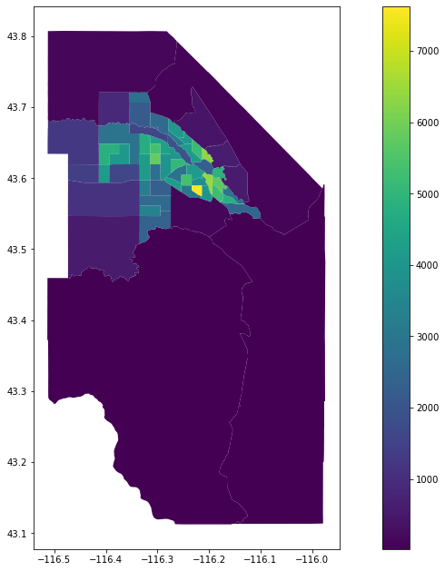

king_pop_tracts=geometrize_census_table_tracts(king['state'],king['county'],get_tract_population(king['state'],king['county']),'Total Population')
king_pop_tracts.plot(column='Density',legend=True,figsize=(17,11))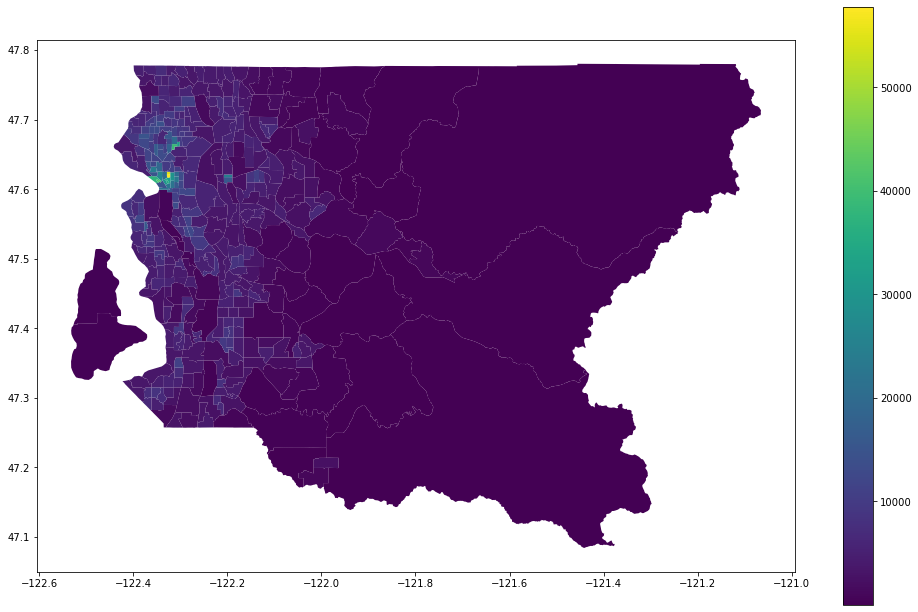

建筑时代的混合 (Mix of Building Ages)

The next most complicated search is to find a variety of building ages within each tract. Luckily, the Census has some data that’s close enough. They track the age of housing within tracts by decade of construction. To start, we’ll make a dictionary out of these table names:

下一个最复杂的搜索是在每个区域中找到各种建筑年龄。 幸运的是，人口普查拥有一些足够接近的数据。 他们通过建造十年来追踪房屋的使用年限。 首先，我们将从这些表名中创建一个字典：

housing_tables={'pre_39':'B25034_011E','1940-1949':'B25034_010E','1950-1959':'B25034_009E','1960-1969':'B25034_008E','1970-1979':'B25034_007E','1980-1989':'B25034_006E','1990-1999':'B25034_005E','2000-2009':'B25034_004E'}

Next, create a function to combine all of these into a single dataframe. Since the Jane-Jacobsy-est tracts will be closest to equal across each decade, the easy metric for this is going to be the standard deviation, with the lowest being best:

接下来，创建一个函数，将所有这些组合到一个数据框中。 由于Jane-Jacobsy-est区域在每个十年中都将最接近相等，因此，最简单的度量标准将是标准差，而最低者为最佳：

def get_housing_age_diversity(state,county):cols=list(housing_tables.keys())cols.insert(0,'TRACTCE10')cols.insert(1,'geometry')out=get_county_tracts(state,county)for key, value in housing_tables.items():out=out.merge(pd.DataFrame(c.acs5.state_county_tract(value,states.lookup(state).fips,county,Census.ALL)),left_on='TRACTCE10',right_on='tract')out.rename(columns={value:key},inplace=True)out=out[cols]out['Standard Deviation']=out.std(axis=1)return out

Again, we simply call our function and plot the results:

同样，我们只需调用函数并绘制结果即可：

ada_housing=get_housing_age_diversity(ada['state'],ada['county'])
ada_housing.plot(column='Standard Deviation',legend=True,figsize=(17,11))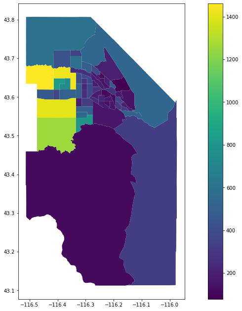

king_housing=get_housing_age_diversity(king['state'],king['county'])
king_housing.plot(column='Standard Deviation',legend=True,figsize=(17,11))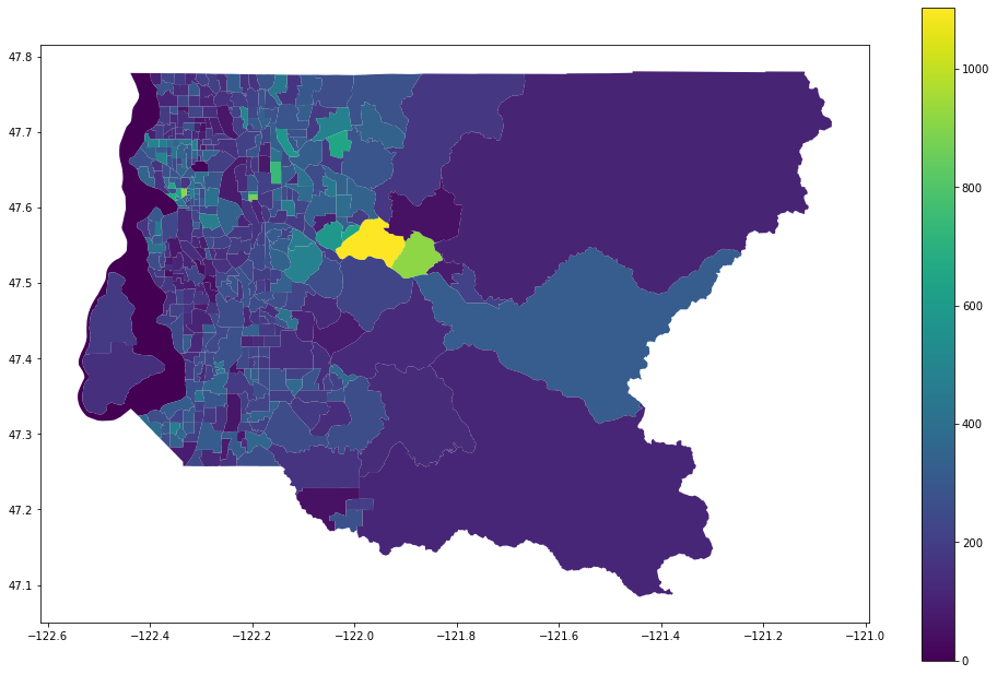

相互连接的短块网络 (A Network of short, interconnected blocks)

Now we start getting complicated. Luckily, we can get a head-start thanks to the osmnx Python package. We’ll use the graph_from_polygon function to get the street network within each Census tract, then the basic_stats package to get the average street length and average number of streets per intersection, or “nodes” in network analysis terms. However, before we do that, we need to fix one problem with our networks: OpenStreetMap counts parking lot drive-aisles as part of the street network, which is going to skew our results, as these tend to be relatively short, and at least connect in the interior of surface parking lots. To fix this, we’ll query all the parking lots in the county, then exclude them from our tracts to get some Swiss cheesy tracts. First, the function to query OSM for stuff, generalized as we’ll be using it heavily in the next section:

现在我们开始变得复杂。 幸运的是， 借助osmnx Python软件包，我们可以抢先一步 。 我们将使用graph_from_polygon函数来获取每个人口普查区域内的街道网络，然后使用basic_stats包来获取平均街道长度和每个路口或网络分析术语中的“节点”的平均街道数。 但是，在执行此操作之前，我们需要解决网络中的一个问题：OpenStreetMap将停车场的驾驶通道算作街道网络的一部分，这会使我们的结果产生偏差，因为这些结果往往相对较短，并且至少连接在地面停车场的内部。 为了解决这个问题，我们将查询该县的所有停车场，然后将其从我们的区域中排除，以获得一些瑞士俗气的区域。 首先，在OSM中查询内容的函数，在下一节中将广泛使用它：

def osm_query(area,elementType,feature_type,feature_name=None,poly_to_point=True):if feature_name:q=overpassQueryBuilder(area=nominatim.query(area).areaId(),elementType=elementType,selector='"{ft}"="{fn}"'.format(ft=feature_type,fn=feature_name),out='body',includeGeometry=True)else:q=overpassQueryBuilder(area=nominatim.query(area).areaId(),elementType=elementType,selector='"{ft}"'.format(ft=feature_type),out='body',includeGeometry=True)if len(overpass.query(q).toJSON()['elements'])>0:out=pd.DataFrame(overpass.query(q).toJSON()['elements'])if elementType=='node':out=gpd.GeoDataFrame(out,geometry=gpd.points_from_xy(out['lon'],out['lat']),crs=wgs)out=out.to_crs(merc)if elementType=='way':geometry=[]for i in out.geometry:geo=osm_way_to_polygon(i)geometry.append(geo)out.geometry=geometryout=gpd.GeoDataFrame(out,crs=wgs)out=out.to_crs(merc)if poly_to_point:out.geometry=out.geometry.centroidout=pd.concat([out.drop(['tags'],axis=1),out['tags'].apply(pd.Series)],axis=1)if elementType=='relation':out=pd.concat([out.drop(['members'],axis=1),out['members'].apply(pd.Series)[0].apply(pd.Series)],axis=1)geometry=[]for index, row in out.iterrows():row['geometry']=osm_way_to_polygon(row['geometry'])geometry.append(row['geometry'])out.geometry=geometryout=gpd.GeoDataFrame(out,crs=wgs)out=out.to_crs(merc)if poly_to_point:out.geometry=out.geometry.centroidout=out[['name','id','geometry']]if feature_name:out['type']= feature_nameelse:out['type']= feature_typeelse:out=pd.DataFrame(columns=['name','id','geometry','type'])return out

To get parking-less tracts:

要获得免停车路段：

ada_tracts=get_county_tracts(ada['state'],ada['county']).to_crs(merc)
ada_parking=osm_query('Ada County, ID','way','amenity','parking',poly_to_point=False)
ada_tracts_parking=gpd.overlay(ada_tracts,ada_parking,how='symmetric_difference')

king_tracts=get_county_tracts(king['state'],king['county']).to_crs(merc)
king_parking=osm_query('king County, WA','way','amenity','parking',poly_to_point=False)
king_tracts_parking=gpd.overlay(king_tracts,king_parking,how='symmetric_difference')

This isn’t going to be a perfect solution as a lot of parking lots aren’t tagged as such, but it will at least exclude a lot of them. Now we can create a function to iterate over each tract and get a “street score” that I’m defining as the average length of streets within the tract divided by the number of streets per intersection:

这并不是一个完美的解决方案，因为许多停车场都没有这样的标签，但至少会排除很多停车场。 现在，我们可以创建一个函数来遍历每个区域并获得“街道分数”，我将其定义为区域内街道的平均长度除以每个路口的街道数量：

def score_streets(gdf):out=gpd.GeoDataFrame()i=1for index, row in gdf.iterrows():try:clear_output(wait=True)g=ox.graph_from_polygon(row['geometry'],network_type='walk')stats=ox.stats.basic_stats(g)row['street_score']=stats['street_length_avg']/stats['streets_per_node_avg']print('{}% complete'.format(round(((i/len(gdf))*100),2)))ox.plot_graph(g,node_size=0)out=out.append(row)i+=1except:continuereturn out

This one takes a while, so I included a progress bar and map output to keep me entertained while I wait There are also some tracts with no streets (I would assume the Puget Sound), hence the try/except. Now we call the function:

这需要一段时间，所以我添加了进度条和地图输出，以使我在等待时保持娱乐。还有一些没有街道的区域(我会假设为普吉特海湾)，因此请尝试/除外。 现在我们调用函数：

ada_street_scores=score_streets(ada_tracts_parking.to_crs(wgs))
ada_street_scores.plot(column='street_score',legend=True,figsize=(17,11))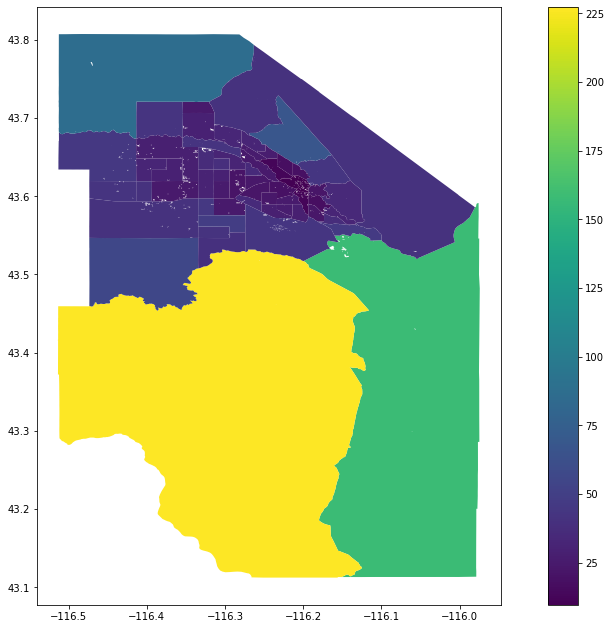

king_street_scores=score_streets(king_tracts_parking.to_crs(wgs))
king_street_scores.plot(column='street_score',legend=True,figsize=(17,11))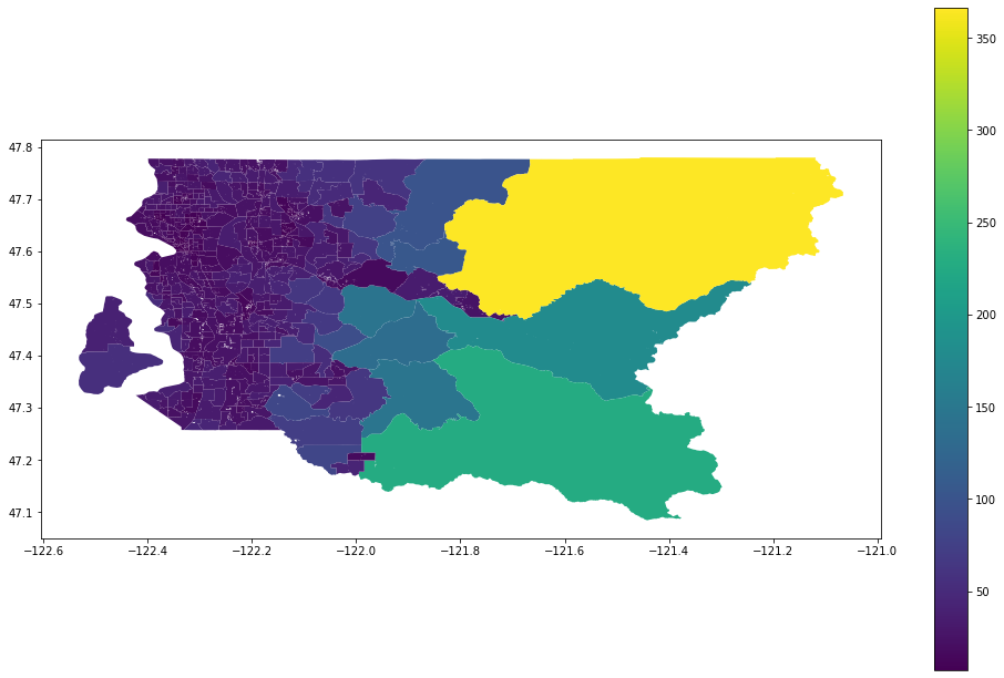

多种用途 (A mix of Uses)

Now for the most complicated portion of the analysis. Here’s my general plan:

现在进行最复杂的分析。 这是我的总体计划：

1. Query OpenStreetMap for all the components of necessary for a “15 minute neighborhood”:查询OpenStreetMap以获取“ 15分钟邻域”所需的所有组件：

• Office办公室
• Park公园
• Bar酒吧
• Restaurant餐厅
• Coffee shop咖啡店
• Library图书馆
• School学校
• Bank银行
• Doctor’s office医生办公室
• Pharmacy药店
• Post office邮政局
• Grocery store杂货店
• Hardware store五金店

2. Get a sample of points within each Census Tract

2.获取每个人口普查区内的点样本

3. Count all the neighborhood essentials within walking distance of each sample point

3.计算每个采样点步行距离内的所有邻域要素

4. Get an average of the number of essentials within walking distance for all the points in the tract.

4.获取该区域中所有点在步行距离内的必需品数量的平均值。

We’ll start with the osm_query function that I used to find parking lots above to get all the neighborhood essentials in a given geography. Since OSM is open source and editable, there are a few quirks to the data to work out. First, some people put point geographies for some things, while others put areas of the buildings. That’s why there’s the poly_to_point option in the function to standardize all of these to points if we want. The raw output of the Overpass API geometry is a dictionary of coordinates, so we need to convert those to shapely geometries in order to get fed into GeoPandas:

我们将从osm_query函数开始，该函数用于查找上方的停车场，以获取给定地理区域中的所有邻域要素。 由于OSM是开源的且可编辑的，因此需要对数据进行一些修改。 首先，有些人对某些事物放置了点地理，而另一些人则对建筑物的区域进行了地理定位。 这就是为什么函数中有poly_to_point选项可以将所有这些标准标准化为点(如果需要)的原因。 Overpass API几何图形的原始输出是一个坐标字典，因此我们需要将其转换为形状几何图形，以便输入到GeoPandas中：

def osm_way_to_polygon(way):points=list()for p in range(len(way)):point=Point(way[p]['lon'],way[p]['lat'])points.append(point)poly=Polygon([[p.x, p.y] for p in points])return poly

We want these to come out in a single column, so we combine the outputs:

我们希望它们在同一列中列出，因此我们将输出合并：

def combine_osm_features(name,feature_type,feature_name=None):df=pd.concat([osm_query(name,'node',feature_type,feature_name),osm_query(name,'way',feature_type,feature_name)])return df

Now we’re finally ready to get our neighborhood essentials:

现在，我们终于准备好获取我们附近的必需品：

def get_key_features(name):df=pd.concat([combine_osm_features(name,'office'),combine_osm_features(name,'leisure','park')])amenities=['bar','restaurant','cafe','library','school','bank','clinic','hospital','pharmacy','post_office']shops=['supermarket','hardware','doityourself']for a in amenities:df=pd.concat([df,combine_osm_features(name,'amenity',a)])for s in shops:df=pd.concat([df,combine_osm_features(name,'shop',s)])df=df.replace('doityourself','hardware')return gpd.GeoDataFrame(df,crs=merc)

Next, we need to get a bunch of random points to search from:

接下来，我们需要从中搜索一堆随机点：

def random_sample_points(poly,npoints=10,tract_col='TRACTCE10'):min_x,min_y,max_x,max_y=poly.geometry.total_boundspoints=[]tracts=[]i=0while i < npoints:point=Point(random.uniform(min_x,max_x),random.uniform(min_y,max_y))if poly.geometry.contains(point).iloc[0]:points.append(point)tracts.append(poly[tract_col].iloc[0])i+=1out=gpd.GeoDataFrame({tract_col:tracts,'geometry':points},crs=poly.crs)return out

Next, we’ll buffer our points by our walkable distance, which I set at 1 km. If we wanted to get really fancy, we’d use walksheds instead, but this analysis is processor heavy enough as it is, so I’m going to opt to stick with euclidian distances. We’ll then grab all the neighborhood essentials within the buffer area, and calculate a percentage of the essentials that are within walking distance:

接下来，我们将根据我们的步行距离(我设定为1公里)缓冲点。 如果我们真的想花哨的话，我们会改用步行棚，但是这种分析实际上要占用大量处理器，因此，我将选择保持欧氏距离。 然后，我们将获取缓冲区内的所有邻近要素，并计算步行距离之内的要素的百分比：

def calculate_nearbyness_tract(tract,features,npoints=10,buffer_dist=1000):points=random_sample_points(tract,npoints).to_crs(merc)points.geometry=points.geometry.buffer(buffer_dist)cols=features['type'].unique().tolist()out=gpd.GeoDataFrame()i=1for index, row in points.iterrows():row['point_id']=ir=gpd.GeoDataFrame(pd.DataFrame(row).T,crs=points.crs,geometry='geometry').to_crs(merc)gdf=gpd.overlay(features,r,how='intersection')out=out.append(gdf)i+=1out=out.groupby(['point_id','type','TRACTCE10'],as_index=False).count()out=out.pivot(['point_id','TRACTCE10'],'type','name')out['nearby']=(out.notnull().sum(axis=1))/len(cols)out=pd.DataFrame(out.mean(axis=0,numeric_only=True)).Tout.insert(0,'tract',tract['TRACTCE10'].iloc[0],True)return out

That gets us the “nearbyness” of one tract. We now need to iterate over all the tracts in the county:

这使我们获得了一个道的“附近”。 现在，我们需要遍历该县的所有区域：

def calculate_nearbyness(gdf,features,npoints=10,buffer_dist=1000):out=pd.DataFrame()cols=features['type'].unique().tolist()for index, row in gdf.iterrows():r=gpd.GeoDataFrame(pd.DataFrame(row).T,crs=gdf.crs,geometry='geometry')near=calculate_nearbyness_tract(r,features,npoints,buffer_dist)out=out.append(near)cols.insert(0,'tract')cols.append('nearby')out.drop(out.columns.difference(cols),1,inplace=True)return out

Now we can call our functions to get our analysis:

现在我们可以调用函数来进行分析：

ada_features=get_key_features(ada['name']).to_crs(merc)
ada_nearby=calculate_nearbyness(ada_tracts,ada_features)
geometrize_census_table_tracts(ada['state'],ada['county'],ada_nearby).plot(column='nearby',legend=True,figsize=(11,17))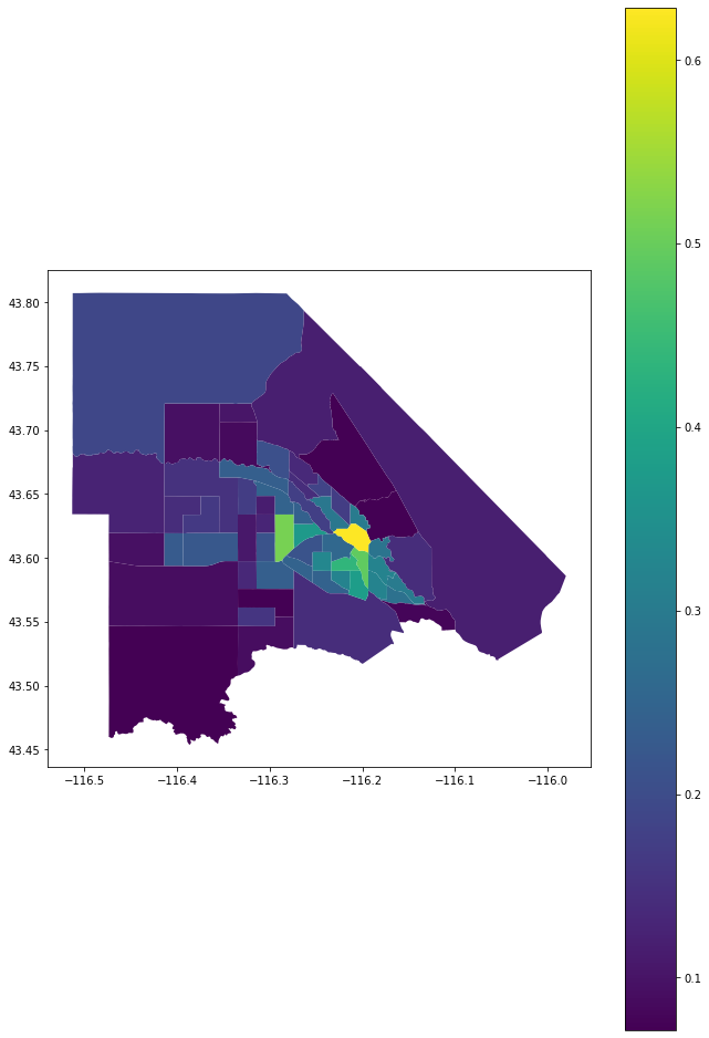

king_features=get_key_features(king['name']).to_crs(merc)
king_nearby=calculate_nearbyness(king_tracts,king_features)
geometrize_census_table_tracts(king['state'],king['county'],king_nearby).plot(column='nearby',legend=True,figsize=(11,17))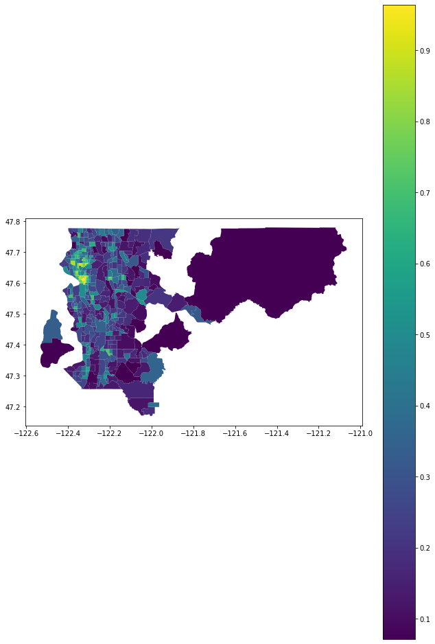

全部放在一起 (Putting it all Together)

We now have a score for each of Jane Jacobs’ factors for a quality neighborhood. I’m more interested in comparing tracts within counties than comparing the counties themselves, so I’m going to simply rank each tract on their scores and take an average to get to the “Jane Jacobs Index” (JJI):

现在，我们为Jane Jacobs的每个优质邻里因素提供了得分。 我对比较县内的地区比对县本身进行比较更感兴趣，因此，我将简单地对每个地区的得分进行排名，并取平均值以得出“简·雅各布斯指数”(JJI)：

def jane_jacobs_index(density,housing_age,mix,streets,merge_col='TRACTCE10'):df=density.merge(housing_age,on=merge_col).merge(mix,on='tract').merge(streets,on=merge_col)df['street_rank']=df['street_score'].rank(ascending=True,na_option='bottom')df['nearby_rank']=df['nearby'].rank(ascending=False,na_option='top')df['housing_rank']=df['Standard Deviation'].rank(ascending=True,na_option='bottom')df['density_rank']=df['Density'].rank(ascending=False,na_option='top')df=df[['TRACTCE10','street_rank','nearby_rank','housing_rank','density_rank']]df['JJI']=df.mean(axis=1)return(df)

To see what we’ve made, we’ll call the function using the four dataframes we made earlier:

为了了解我们所做的事情，我们将使用我们之前制作的四个数据框来调用该函数：

ada_jji=jane_jacobs_index(ada_pop_tracts,ada_housing,ada_nearby,ada_street_scores)
ada_jji=geometrize_census_table_tracts(ada['state'],ada['county'],ada_jji,right_on='TRACTCE10')
ada_jji.plot(column='JJI',legend=True, figsize=(17,11))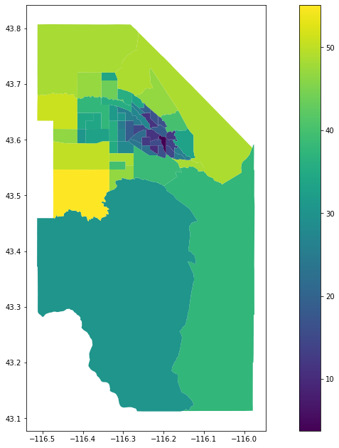

king_jji=jane_jacobs_index(king_pop_tracts,king_housing,king_nearby,king_street_scores)
king_jji=geometrize_census_table_tracts(king['state'],king['county'],king_jji,right_on='TRACTCE10')
king_jji.plot(column='JJI',legend=True, figsize=(17,11))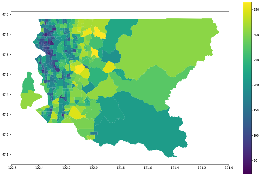

Finally, for cool points, we’ll use Folium to create an interactive map:

最后，对于酷点，我们将使用Folium创建一个交互式地图：

ada_map=folium.Map(location=[43.4595119,-116.524329],zoom_start=10)
folium.Choropleth(geo_data=ada_jji,data=ada_jji,columns=['TRACTCE10','JJI'],fill_color='YlGnBu',key_on='feature.properties.TRACTCE10',highlight=True,name='Jane Jacobs Index',legend_name='Jane Jacobs Index',line_weight=.2).add_to(ada_map)
folium.Choropleth(geo_data=ada_jji,data=ada_jji,columns=['TRACTCE10','street_rank'],fill_color='YlGnBu',key_on='feature.properties.TRACTCE10',highlight=True,show=False,name='Street Rank',legend_name='Street Rank',line_weight=.2).add_to(ada_map)
folium.Choropleth(geo_data=ada_jji,data=ada_jji,columns=['TRACTCE10','nearby_rank'],fill_color='YlGnBu',key_on='feature.properties.TRACTCE10',highlight=True,show=False,name='Nearby Rank',legend_name='Nearby Rank',line_weight=.2).add_to(ada_map)
folium.Choropleth(geo_data=ada_jji,data=ada_jji,columns=['TRACTCE10','housing_rank'],fill_color='YlGnBu',key_on='feature.properties.TRACTCE10',highlight=True,show=False,name='Housing Age Rank',legend_name='Housing Age Rank',line_weight=.2).add_to(ada_map)
folium.Choropleth(geo_data=ada_jji,data=ada_jji,columns=['TRACTCE10','density_rank'],fill_color='YlGnBu',key_on='feature.properties.TRACTCE10',highlight=True,show=False,name='Density Rank',legend_name='Density Rank',line_weight=.2).add_to(ada_map)
folium.LayerControl(collapsed=False).add_to(ada_map)
ada_map.save('ada_map.html')

king_map=folium.Map(location=[47.4310271,-122.3638018],zoom_start=9)
folium.Choropleth(geo_data=king_jji,data=king_jji,columns=['TRACTCE10','JJI'],fill_color='YlGnBu',key_on='feature.properties.TRACTCE10',highlight=True,name='Jane Jacobs Index',legend_name='Jane Jacobs Index',line_weight=.2).add_to(king_map)
folium.Choropleth(geo_data=king_jji,data=king_jji,columns=['TRACTCE10','street_rank'],fill_color='YlGnBu',key_on='feature.properties.TRACTCE10',highlight=True,show=False,name='Street Rank',legend_name='Street Rank',line_weight=.2).add_to(king_map)
folium.Choropleth(geo_data=king_jji,data=king_jji,columns=['TRACTCE10','nearby_rank'],fill_color='YlGnBu',key_on='feature.properties.TRACTCE10',highlight=True,show=False,name='Nearby Rank',legend_name='Nearby Rank',line_weight=.2).add_to(king_map)
folium.Choropleth(geo_data=king_jji,data=king_jji,columns=['TRACTCE10','housing_rank'],fill_color='YlGnBu',key_on='feature.properties.TRACTCE10',highlight=True,show=False,name='Housing Age Rank',legend_name='Housing Age Rank',line_weight=.2).add_to(king_map)
folium.Choropleth(geo_data=king_jji,data=king_jji,columns=['TRACTCE10','density_rank'],fill_color='YlGnBu',key_on='feature.properties.TRACTCE10',highlight=True,show=False,name='Density Rank',legend_name='Density Rank',line_weight=.2).add_to(king_map)
folium.LayerControl(collapsed=False).add_to(king_map)
king_map.save('king_map.html')

Here are links to the two newly created maps:

这是两个新创建的地图的链接：

Ada County

阿达县

King County

金县

What’s it all mean? We’ll dive into that in Part II…

什么意思 我们将在第二部分中深入探讨……