数据科学 ， 机器学习 (Data Science, Machine Learning)

前言 (Preface)

Cardiovascular diseases are diseases of the heart and blood vessels and they typically include heart attacks, strokes, and heart failures [1]. According to the World Health Organization (WHO), cardiovascular diseases like ischaemic heart disease and stroke have been the leading causes of deaths worldwide for the last decade and a half [2].

心血管疾病是心脏和血管疾病，通常包括心脏病发作，中风和心力衰竭[1]。 根据世界卫生组织(WHO)的研究，在过去的15年中，缺血性心脏病和中风等心血管疾病已成为全球死亡的主要原因[2]。

动机 (Motivation)

A few months ago, a new heart failure dataset was uploaded on Kaggle. This dataset contained health records of 299 anonymized patients and had 12 clinical and lifestyle features. The task was to predict heart failure using these features.

几个月前，一个新的心力衰竭数据集被上传到Kaggle上 。 该数据集包含299名匿名患者的健康记录，并具有12种临床和生活方式特征。 他们的任务是使用这些功能来预测心力衰竭。

Through this post, I aim to document my workflow on this task and present it as a research exercise. So this would naturally involve a bit of domain knowledge, references to journal papers, and deriving insights from them.

通过这篇文章，我旨在记录我有关此任务的工作流程，并将其作为研究练习进行介绍。 因此，这自然会涉及到一些领域知识，对期刊论文的引用以及从中得出的见解。

Warning: This post is nearly 10 minutes long and things may get a little dense as you scroll down, but I encourage you to give it a shot.

警告：这篇文章将近10分钟，当您向下滚动时，内容可能会变得有些密集，但我建议您试一试。

关于数据 (About the data)

The dataset was originally released by Ahmed et al., in 2017 [3] as a supplement to their analysis of survival of heart failure patients at Faisalabad Institute of Cardiology and at the Allied Hospital in Faisalabad, Pakistan. The dataset was subsequently accessed and analyzed by Chicco and Jurman in 2020 to predict heart failures using a bunch of machine learning techniques [4]. The dataset hosted on Kaggle cites these authors and their research paper.

该数据集最初由Ahmed等人在2017年发布[3]，作为他们对巴基斯坦费萨拉巴德心脏病研究所和联合王国费萨拉巴德联合医院心力衰竭患者生存率分析的补充。 随后，Chicco和Jurman于2020年访问并分析了该数据集，以使用一系列机器学习技术预测心力衰竭[4]。 Kaggle托管的数据集引用了这些作者及其研究论文。

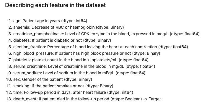
The dataset primarily consists of clinical and lifestyle features of 105 female and 194 male heart failure patients. You can find each feature explained in the figure below.

该数据集主要由105位女性和194位男性心力衰竭患者的临床和生活方式特征组成。 您可以找到下图中说明的每个功能。

项目工作流程 (Project Workflow)

The workflow would be pretty straightforward —

工作流程将非常简单-

1. Data Preprocessing — Cleaning the data, imputing missing values, creating new features if needed, etc.

   数据预处理-清理数据，估算缺失值，根据需要创建新功能等。

2. Exploratory Data Analysis — This would involve summary statistics, plotting relationships, mapping trends, etc.

   探索性数据分析-这将涉及摘要统计，绘制关系，绘制趋势等。

3. Model Building — Building a baseline prediction model, followed by at least 2 classification models to train and test.

   建立模型—建立基线预测模型，然后建立至少两个分类模型以进行训练和测试。

4. Hyper-parameter Tuning — Fine-tune the hyper-parameters of each model to arrive at acceptable levels of prediction metrics.

   超参数调整-微调每个模型的超参数，以达到可接受的预测指标水平。

5. Consolidating Results — Presenting relevant findings in a clear and concise manner.

   合并结果—清晰，简明地陈述相关发现。

The entire project can be found as a Jupyter notebook on my GitHub repository.

整个项目都可以在我的 GitHub 存储库中 找到，作为Jupyter笔记本 。

让我们开始！ (Let’s begin!)

数据预处理 (Data Preprocessing)

Let’s read in the .csv file into a dataframe —

让我们将.csv文件读入数据框-

df = pd.read_csv('heart_failure_clinical_records_dataset.csv')

df.info() is a quick way to get a summary of the dataframe data types. We see that the dataset has no missing or spurious values and is clean enough to begin data exploration.

df.info()是获取数据框数据类型摘要的快速方法。 我们看到数据集没有丢失或伪造的值，并且足够干净以开始数据探索。

<class 'pandas.core.frame.DataFrame'>RangeIndex: 299 entries, 0 to 298Data columns (total 13 columns): #   Column                    Non-Null Count  Dtype  ---  ------                    --------------  -----   0   age                       299 non-null    float64 1   anaemia                   299 non-null    int64   2   creatinine_phosphokinase  299 non-null    int64   3   diabetes                  299 non-null    int64   4   ejection_fraction         299 non-null    int64   5   high_blood_pressure       299 non-null    int64   6   platelets                 299 non-null    float64 7   serum_creatinine          299 non-null    float64 8   serum_sodium              299 non-null    int64   9   sex                       299 non-null    int64   10  smoking                   299 non-null    int64   11  time                      299 non-null    int64   12  DEATH_EVENT               299 non-null    int64  dtypes: float64(3), int64(10)memory usage: 30.5 KB

But before that, let us rearrange and rename some of the features, add another feature called chk(which would be useful later during EDA) and replace the binary values in the categorical features with their labels (again, useful during EDA).

但是在此之前，让我们重新排列并重命名一些功能，添加另一个名为chk功能( 在EDA中稍后会 chk )，然后用其标签替换分类功能中的二进制值( 再次在EDA中使用 )。

df = df.rename(columns={'smoking':'smk',                        'diabetes':'dia',                        'anaemia':'anm',                        'platelets':'plt',                        'high_blood_pressure':'hbp',                        'creatinine_phosphokinase':'cpk',                        'ejection_fraction':'ejf',                        'serum_creatinine':'scr',                        'serum_sodium':'sna',                        'DEATH_EVENT':'death'})df['chk'] = 1df['sex'] = df['sex'].apply(lambda x: 'Female' if x==0 else 'Male')df['smk'] = df['smk'].apply(lambda x: 'No' if x==0 else 'Yes')df['dia'] = df['dia'].apply(lambda x: 'No' if x==0 else 'Yes')df['anm'] = df['anm'].apply(lambda x: 'No' if x==0 else 'Yes')df['hbp'] = df['hbp'].apply(lambda x: 'No' if x==0 else 'Yes')df['death'] = df['death'].apply(lambda x: 'No' if x==0 else 'Yes')df.info()<class 'pandas.core.frame.DataFrame'>RangeIndex: 299 entries, 0 to 298Data columns (total 14 columns): #   Column  Non-Null Count  Dtype  ---  ------  --------------  -----   0   sex     299 non-null    object  1   age     299 non-null    float64 2   smk     299 non-null    object  3   dia     299 non-null    object  4   hbp     299 non-null    object  5   anm     299 non-null    object  6   plt     299 non-null    float64 7   ejf     299 non-null    int64   8   cpk     299 non-null    int64   9   scr     299 non-null    float64 10  sna     299 non-null    int64   11  time    299 non-null    int64   12  death   299 non-null    object  13  chk     299 non-null    int64  dtypes: float64(3), int64(5), object(6)memory usage: 32.8+ KB

We observe that sex, dia, anm, hbp, smk anddeathare categorical features (object), while age, plt,cpk, ejf, scr, timeand sna are numerical features (int64 or float64). All features except death would be potential predictors and death would be the target for our prospective ML model.

我们观察到， sex ， dia ， anm ， hbp ， smk和death的类别特征( 对象 )，而age ， plt ， cpk ， ejf ， scr ， time和sna的数字功能(Int64的或float64)。 除death以外的所有功能都是潜在的预测因素，而death将成为我们预期的ML模型的目标。

探索性数据分析 (Exploratory Data Analysis)

A.数值特征汇总统计 (A. Summary Statistics of Numerical Features)

Since our dataset has many numerical features, it would be helpful to look at some aggregate measures of the data in hand, with the help of df.describe() (Usually, this method gives values up to 6 decimal places, so it would better to round it off to two by df.describe().round(2))

由于我们的数据集具有许多数值特征，因此在df.describe()的帮助下df.describe()手头数据的一些聚合度量将很有帮助( 通常，此方法最多可提供小数点后6位的值，因此最好到轮它关闭两个由 df.describe().round(2)

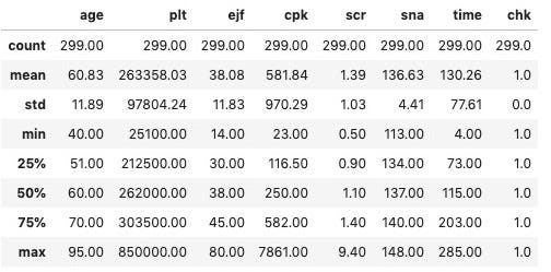
• Age: We can see that the average age of the patients is 60 years with most of the patients (<75%) below 70 years and above 40 years. The follow-up time after their heart failure also varies from 4 days to 285 days, with an average of 130 days.

  年龄 ：我们可以看到患者的平均年龄为60岁，其中大多数患者(<75％)低于70岁且高于40岁。 他们心力衰竭后的随访时间也从4天到285天不等，平均为130天。

• Platelets: These are a type of blood cells that are responsible for repairing damaged blood vessels. A normal person has a platelet count of 150,000–400,000 kiloplatelets/mL of blood [5]. In our dataset, 75% of the patients have a platelet count well within this range.

  血小板 ： 血小板 是负责修复受损血管的一种血细胞。 正常人的血小板计数为150,000–400,000血小板/ mL血液[5]。 在我们的数据集中，有75％的患者血小板计数在此范围内。

• Ejection fraction: This is a measure (in %) of how much blood is pumped out of a ventricle in each contraction. To brush up a little human anatomy — the heart has 4 chambers of which the atria receive blood from different parts of the body and the ventricles pump it to back. The left ventricle is the thickest chamber and pumps blood to the rest of the body while the right ventricle pumps blood to the lungs. In a healthy adult, this fraction is 55% and heart failure with reduced ejection fraction implies a value < 40%[6]. In our dataset, 75% of the patients have this value < 45% which is expected because they are all heart failure patients in the first place.

  射血分数 ： 这是每次收缩中从脑室中抽出多少血液的量度(％)。 为了梳理一点人体解剖学，心脏有4个腔室，心房从身体的不同部位接收血液，心室将其泵回。 左心室是最厚的腔室，将血液泵送到身体的其余部分，而右心室则将血液泵到肺。 在健康的成年人中，这一比例为55％，而射血分数降低的心力衰竭意味着其值<40％[6]。 在我们的数据集中，有75％的患者的此值<45％ ，这是可以预期的，因为他们首先都是心力衰竭患者。

• Creatinine Phosphokinase: This is an enzyme that is present in the blood and helps in repairing damaged tissues. A high level of CPK implies heart failure or injury. The normal levels in males are 55–170 mcg/L and in females are 30–135 mcg/L [7]. In our dataset, since all patients have had heart failure, the average value (550 mcg/L) and median (250 mcg/L) are higher than normal.

  肌酐磷酸激酶 ： 这是一种存在于血液中的酶，有助于修复受损的组织。 高水平的CPK意味着心力衰竭或伤害。 男性的正常水平为55–170 mcg / L，女性为30–135 mcg / L [7]。 在我们的数据集中，由于所有患者都患有心力衰竭， 因此平均值(550 mcg / L)和中位数(250 mcg / L)高于正常水平。

• Serum creatinine: This is a waste product that is produced as a part of muscle metabolism especially during muscle breakdown. This creatinine is filtered by the kidneys and increased levels are indicative of poor cardiac output and possible renal failure[8]. The normal levels are between 0.84 to 1.21 mg/dL [9] and in our dataset, the average and median are above 1.10 mg/dL, which is pretty close to the upper limit of the normal range.

  血清肌酐 ： 这是一种废物，是肌肉代谢的一部分，特别是在肌肉分解过程中。 肌酐被肾脏过滤，水平升高表明心输出量不良和可能的肾衰竭 [8]。 正常水平在0.84至1.21 mg / dL之间[9]，在我们的数据集中，平均值和中位数高于1.10 mg / dL， 非常接近正常范围的上限 。

• Serum sodium: This refers to the level of sodium in the blood and a high level of > 135 mEq/L is called hypernatremia, which is considered typical in heart failure patients [10]. In our dataset, we find that the average and the median are > 135 mEq/L.

  血清钠 ： 指血液中的钠水平，> 135 mEq / L的高水平被称为高钠血症，在心力衰竭患者中被认为是典型的 [10]。 在我们的数据集中，我们发现平均值和中位数> 135 mEq / L。

A neat way to visualize these statistics is with a boxenplot which shows the spread and distribution of values (The line in the center is the median and the diamonds at the end are the outliers).

直观显示这些统计数据的一种好方法是使用boxenplot ，该boxenplot显示值的分布和分布( 中间的线是中位数，而末端的菱形是异常值 )。

fig,ax = plt.subplots(3,2,figsize=[10,10])num_features_set1 = ['age', 'scr', 'sna']num_features_set2 = ['plt', 'ejf', 'cpk']for i in range(0,3):    sns.boxenplot(df[num_features_set1[i]], ax=ax[i,0], color='steelblue')    sns.boxenplot(df[num_features_set2[i]], ax=ax[i,1], color='steelblue')

B.分类特征摘要统计 (B. Summary Statistics of Categorical Features)

The number of patients belonging to each of the lifestyle categorical features can be summarised with a simple bar plot .

可以通过简单的bar plot总结属于每种生活方式分类特征的患者人数。

fig = plt.subplots(figsize=[10,6])bar1 = df.smk.value_counts().valuesbar2 = df.hbp.value_counts().valuesbar3 = df.dia.value_counts().valuesbar4 = df.anm.value_counts().valuesticks = np.arange(0,3, 2)width = 0.3plt.bar(ticks, bar1, width=width, color='teal', label='smoker')plt.bar(ticks+width, bar2, width=width, color='darkorange', label='high blood pressure')plt.bar(ticks+2*width, bar3, width=width, color='limegreen', label='diabetes')plt.bar(ticks+3*width, bar4, width=width, color='tomato', label='anaemic')plt.xticks(ticks+1.5*width, ['Yes', 'No'])plt.ylabel('Number of patients')plt.legend()

Additional summaries can be generated using the crosstab function in pandas. An example is shown for the categorical feature smk . The results can be normalized with respect to either the total number of smokers (‘index’) or the total number of deaths (‘columns’). Since our interest is in predicting survival, we normalize with respect to death.

可以使用pandas中的crosstab功能生成其他摘要。 显示了分类特征smk的示例。 可以根据吸烟者总数( “指数” )或死亡总数( “列” )对结果进行标准化。 由于我们的兴趣在于预测生存，因此我们将死亡归一化。

pd.crosstab(index=df['smk'], columns=df['death'], values=df['chk'], aggfunc=np.sum, margins=True)pd.crosstab(index=df['smk'], columns=df['death'], values=df['chk'], aggfunc=np.sum, margins=True, normalize='columns').round(2)*100

We see that 68% of all heart failure patients did not smoke while 32% did. Of those who died, 69% were non-smokers while 31% were smokers. Of those who survived, 67% were non-smokers and 33% were smokers. At this point, it is difficult to say, conclusively, that heart failure patients who smoked have a greater chance of dying.

我们发现68％的心力衰竭患者不吸烟，而32％的人吸烟。 在死亡者中 ，不吸烟者占69％，吸烟者占31％。 在幸存者中 ，不吸烟者占67％，吸烟者占33％。 在这一点上，很难说得出结论，吸烟的心力衰竭患者死亡的机会更大。

In a similar manner, let’s summarise the rest of the categorical features and normalize the results with respect to deaths.

以类似的方式，让我们总结一下其余的分类特征，并就死亡对结果进行归一化。

• 65% of the Male and 35% of the Female heart patients died.65％的男性心脏病患者和35％的女性心脏病患者死亡。
• 48% of the patients who died were anemic while 41% of the patients who survived were anemic as well.死亡的患者中有48％贫血，而幸存的患者中有41％贫血。
• 42% of the patients who died and 42% who survived were diabetic.42％的死亡患者和42％的幸存者患有糖尿病。
• 31% of the dead were smokers while 33% of the survivors were smokers.死者中有31％是吸烟者，而幸存者中有33％是吸烟者。
• 41% of those who died had high blood pressure, while 33% of those who survived had high blood pressure as well.死者中有41％患有高血压，而幸存者中有33％患有高血压。

Based on these statistics, we get a rough idea that the lifestyle features are almost similarly distributed amongst those who died and those who survived. The difference is the greatest in the case of high blood pressure, which could perhaps have a greater influence on the survival of heart patients.

根据这些统计数据，我们可以粗略了解一下，生活方式特征在死者和幸存者之间的分布几乎相似。 在高血压的情况下，差异最大，这可能对心脏病患者的生存产生更大的影响。

C.探索数字特征之间的关系 (C. Exploring relationships between numerical features)

The next step is to visualize the relationship between features. We start with the numerical features by writing a single line of code to plot a pair-wise plotting of features using seaborn’s pairplot—

下一步是可视化要素之间的关系。 我们从数字特征开始，编写一行代码以使用seaborn的对图绘制特征的pairplot ，

sns.pairplot(df[['plt', 'ejf', 'cpk', 'scr', 'sna', 'death']],              hue='death', palette='husl', corner=True)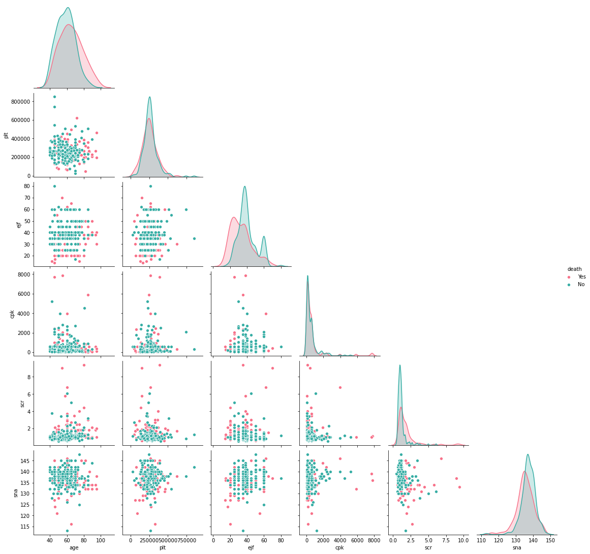

We observe a few interesting points —

我们观察到一些有趣的观点-

• Most of the patients who died following a heart failure seem to have a lower Ejection Fraction that those who survived. They also seem to have slightly higher levels of Serum Creatinine and Creatine Phosphokinase. They also tend to be on the higher side of 80 years.死于心力衰竭的大多数患者的射血分数似乎比那些幸存者低。 他们的血清肌酐和肌酸磷酸激酶水平似乎也略高。 他们也往往处于80年的较高地位。

• There are no strong correlations between features and this can be validated by calculating the Spearman R correlation coefficient (We consider the spearman because we are not sure about the population distribution from which the feature values are drawn).

  特征之间没有很强的相关性，可以通过计算Spearman R相关系数来验证( 我们考虑使用spearman，因为我们不确定从中得出特征值的总体分布 )。

df[['plt', 'ejf', 'cpk', 'scr', 'sna']].corr(method='spearman')

• As observed, the correlation coefficients are moderately encouraging for age-serum creatinine and serum creatinine-serum sodium. From literature, we see that with age, the serum creatinine content increases [11], which explains their slightly positive relationship. Literature also tells us [12] that the sodium to serum creatinine ratio is high in the case of chronic kidney disease which implies a negative relationship between the two. The slight negative correlation coefficient also implies the prevalence of renal issues in the patients.

  如观察到的， 年龄-血清肌酐和血清肌酐-血清钠的相关系数适度令人鼓舞 。 从文献中我们看到，随着年龄的增长，血清肌酐含量增加[11]，这说明了它们之间的正相关关系 。 文献还告诉我们[12]，在慢性肾脏疾病的情况下，钠与血清肌酐的比例较高，这意味着两者之间存在负相关关系 。 轻微的负相关系数也意味着患者中肾脏疾病的患病率。

D.探索分类特征之间的关系 (D. Exploring relationships between categorical features)

One way of relating categorical features is to create a pivot table and pivot about a subset of the features. This would give us the number of values for a particular subset of feature values. For this dataset, let’s look at the lifestyle features — smoking, anemic, high blood pressure, and diabetes.

一种关联分类要素的方法是创建数据透视表并围绕要素的子集进行透视。 这将为我们提供特征值特定子集的值数量。 对于此数据集，让我们看一下生活方式特征-吸烟，贫血，高血压和糖尿病。

lifestyle_surv = pd.pivot_table(df.loc[df.death=='No'],                                 values='chk',                                 columns=['hbp','dia'],                                 index=['smk','anm'],                                 aggfunc=np.sum)lifestyle_dead = pd.pivot_table(df.loc[df.death=='Yes'],                                 values='chk',                                 columns=['hbp','dia'],                                 index=['smk','anm'],                                 aggfunc=np.sum)fig, ax= plt.subplots(1, 2, figsize=[15,6])sns.heatmap(lifestyle_surv, cmap='Greens', annot=True, ax=ax[0])ax[0].set_title('Survivors')sns.heatmap(lifestyle_dead, cmap='Reds', annot=True, ax=ax[1])ax[1].set_title('Deceased')

A few insights can be drawn —

可以得出一些见解-

• A large number of the patients did not smoke, were not anemic and did not suffer from high blood pressure or diabetes.许多患者不吸烟，没有贫血，没有高血压或糖尿病。
• There were very few patients who had all the four lifestyle features.具有这四种生活方式特征的患者很少。
• Many of the survivors were either only smokers or only diabetic.许多幸存者要么只是吸烟者，要么只是糖尿病患者。
• The majority of the deceased had none of the lifestyle features, or at the most were anemic.死者中大多数没有生活方式特征，或者最多是贫血。
• Many of the deceased were anemic and diabetic as well.许多死者也是贫血和糖尿病患者。

E.探索所有功能之间的关系 (E. Exploring relationships between all features)

An easy way to combine categorical and numerical features into a single graph is bypassing the categorical feature as a hue input. In this case, we use the binary death feature and plot violin-plots to visualize the relationships across all features.

将分类特征和数字特征组合到单个图形中的一种简单方法是绕过分类特征作为hue输入。 在这种情况下，我们使用二进制death特征并绘制小提琴图以可视化所有特征之间的关系。

fig,ax = plt.subplots(6, 5, figsize=[20,22])cat_features = ['sex','smk','anm', 'dia', 'hbp']num_features = ['age', 'scr', 'sna', 'plt', 'ejf', 'cpk']for i in range(0,6):    for j in range(0,5):        sns.violinplot(data=df, x=cat_features[j],y=num_features[i], hue='death', split=True, palette='husl',facet_kws={'despine':False}, ax=ax[i,j])        ax[i,j].legend(title='death', loc='upper center')

Here are a few insights from these plots —

以下是这些图的一些见解-

• Sex: Of the patients who died, the ejection fraction seems to be lower in males than in females. Also, the creatinine phosphokinase seems to be higher in males than in females.

  性别 ：在死亡的患者中，男性的射血分数似乎低于女性。 另外，男性的肌酐磷酸激酶似乎高于女性。

• Smoking: A slightly lower ejection fraction was seen in the smokers who died than in the non-smokers who died. The creatinine phosphokinase levels seem to be higher in smokers who survived, than in non-smokers who survived.

  吸烟 ：死亡的吸烟者的射血分数比未死亡的非吸烟者略低。 存活的吸烟者的肌酐磷酸激酶水平似乎高于存活的非吸烟者。

• Anemia: The anemic patients tend to have lower creatinine phosphokinase levels and higher serum creatinine levels, than non-anemic patients. Among the anemic patients, the ejection fraction is lower in those who died than in those who survived.

  贫血 ：与非贫血患者相比，贫血患者的肌酐磷酸激酶水平和血清肌酐水平较高。 在贫血患者中，死亡者的射血分数低于幸存者。

• Diabetes: The diabetic patients tend to have lower sodium levels and again, the ejection fraction is lower in those who died than in the survivors.

  糖尿病 ：糖尿病患者的钠水平较低，而且死亡者的射血分数比幸存者低。

• High Blood Pressure: The ejection fraction seems to show greater variation in deceased patients with high blood pressure than in deceased patients without high blood pressure.

  高血压 ：高血压的死者的射血分数似乎比没有高血压的死者更大。

I hope you found this useful. The steps for building ML models, tuning their hyper-parameters, and consolidating the results will be shown in the next post.

希望您觉得这有用。 建立ML模型，调整其超参数以及合并结果的步骤将在下一篇文章中显示。

Ciao!

再见！