Multivariate Time Series Analysis

多元时间序列分析

A univariate time series data contains only one single time-dependent variable while a multivariate time series data consists of multiple time-dependent variables. We generally use multivariate time series analysis to model and explain the interesting interdependencies and co-movements among the variables. In the multivariate analysis — the assumption is that the time-dependent variables not only depend on their past values but also show dependency between them. Multivariate time series models leverage the dependencies to provide more reliable and accurate forecasts for a specific given data, though the univariate analysis outperforms multivariate in general[1]. In this article, we apply a multivariate time series method, called Vector Auto Regression (VAR) on a real-world dataset.

单变量时间序列数据仅包含一个时间相关的变量，而多元时间序列数据则包含多个时间相关的变量。 我们通常使用多元时间序列分析来建模和解释变量之间有趣的相互依存关系和共同运动。 在多变量分析中，假定时间相关变量不仅取决于它们的过去值，而且还显示它们之间的依赖关系。 多元时间序列模型利用依存关系为特定的给定数据提供更可靠，更准确的预测，尽管单变量分析通常优于多元变量[1]。 在本文中，我们在现实世界的数据集上应用了一种称为向量自动回归(VAR)的多元时间序列方法。

Vector Auto Regression (VAR)

向量自回归(VAR)

VAR model is a stochastic process that represents a group of time-dependent variables as a linear function of their own past values and the past values of all the other variables in the group.

VAR模型是一个随机过程，将一组时间相关变量表示为它们自己的过去值以及该组中所有其他变量的过去值的线性函数。

For instance, we can consider a bivariate time series analysis that describes a relationship between hourly temperature and wind speed as a function of past values [2]:

例如，我们可以考虑一个双变量时间序列分析，该分析描述了每小时温度和风速之间的关系，该关系是过去值的函数[2]：

temp(t) = a1 + w11* temp(t-1) + w12* wind(t-1) + e1(t-1)

temp(t)= a1 + w11 * temp(t-1)+ w12 * wind(t-1)+ e1(t-1)

wind(t) = a2 + w21* temp(t-1) + w22*wind(t-1) +e2(t-1)

wind(t)= a2 + w21 * temp(t-1)+ w22 * wind(t-1)+ e2(t-1)

where a1 and a2 are constants; w11, w12, w21, and w22 are the coefficients; e1 and e2 are the error terms.

其中a1和a2是常数； w11，w12，w21和w22是系数； e1和e2是误差项。

Dataset

数据集

Statmodels is a python API that allows users to explore data, estimate statistical models, and perform statistical tests [3]. It contains time series data as well. We download a dataset from the API.

Statmodels是python API，允许用户浏览数据，估计统计模型并执行统计测试[3]。 它还包含时间序列数据。 我们从API下载数据集。

To download the data, we have to install some libraries and then load the data:

要下载数据，我们必须安装一些库，然后加载数据：

import pandas as pdimport statsmodels.api as smfrom statsmodels.tsa.api import VARdata = sm.datasets.macrodata.load_pandas().datadata.head(2)

The output shows the first two observations of the total dataset:

输出显示了总数据集的前两个观察值：

The data contains a number of time-series data, we take only two time-dependent variables “realgdp” and “realdpi” for experiment purposes and use “year” columns as the index of the data.

数据包含许多时间序列数据，出于实验目的，我们仅采用两个与时间相关的变量“ realgdp”和“ realdpi”，并使用“ year”列作为数据索引。

data1 = data[["realgdp", 'realdpi']]data1.index = data["year"]

output:

输出：

Let's visualize the data:

让我们可视化数据：

data1.plot(figsize = (8,5))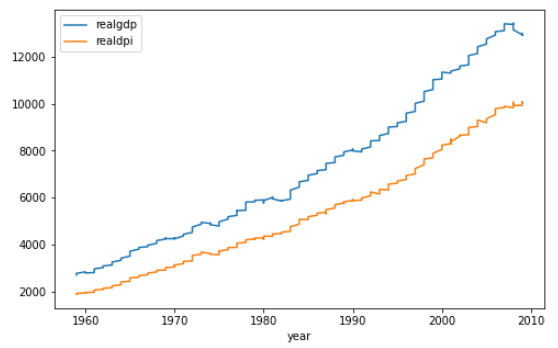

Both of the series show an increasing trend over time with slight ups and downs.

这两个系列都显示出随着时间的推移呈上升趋势，并有轻微的起伏。

Stationary

固定式

Before applying VAR, both the time series variable should be stationary. Both the series are not stationary since both the series do not show constant mean and variance over time. We can also perform a statistical test like the Augmented Dickey-Fuller test (ADF) to find stationarity of the series using the AIC criteria.

应用VAR之前，两个时间序列变量均应为固定值。 两个序列都不是平稳的，因为两个序列都没有显示出恒定的均值和随时间变化。 我们还可以执行统计测试(如增强迪基-富勒检验(ADF))，以使用AIC标准查找系列的平稳性。

adfuller_test = adfuller(data1['realgdp'], autolag= "AIC")print("ADF test statistic: {}".format(adfuller_test[0]))print("p-value: {}".format(adfuller_test[1]))

output:

输出：

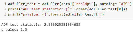
In both cases, the p-value is not significant enough, meaning that we can not reject the null hypothesis and conclude that the series are non-stationary.

在这两种情况下，p值都不足够显着，这意味着我们不能拒绝原假设并得出结论该序列是非平稳的。

Differencing

差异化

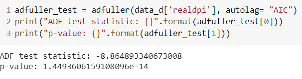
As both the series are not stationary, we perform differencing and later check the stationarity.

由于两个系列都不平稳，因此我们进行微分，然后检查平稳性。

data_d = data1.diff().dropna()

The “realgdp” series becomes stationary after first differencing of the original series as the p-value of the test is statistically significant.

由于测试的p值具有统计意义，因此“ realgdp”系列在对原始系列进行第一次求差后将变得平稳。

The “realdpi” series becomes stationary after first differencing of the original series as the p-value of the test is statistically significant.

由于原始的p值在统计上具有显着性，因此“ realdpi”系列在与原始系列进行首次差异化处理后就变得稳定了。

Model

模型

In this section, we apply the VAR model on the one differenced series. We carry-out the train-test split of the data and keep the last 10-days as test data.

在本节中，我们将VAR模型应用于一个差分序列。 我们对数据进行火车测试拆分，并保留最后10天作为测试数据。

train = data_d.iloc[:-10,:]test = data_d.iloc[-10:,:]

Searching optimal order of VAR model

搜索VAR模型的最优阶

In the process of VAR modeling, we opt to employ Information Criterion Akaike (AIC) as a model selection criterion to conduct optimal model identification. In simple terms, we select the order (p) of VAR based on the best AIC score. The AIC, in general, penalizes models for being too complex, though the complex models may perform slightly better on some other model selection criterion. Hence, we expect an inflection point in searching the order (p), meaning that, the AIC score should decrease with order (p) gets larger until a certain order and then the score starts increasing. For this, we perform grid-search to investigate the optimal order (p).

在VAR建模过程中，我们选择采用信息准则赤池(AIC)作为模型选择标准来进行最佳模型识别。 简单来说，我们根据最佳AIC得分选择VAR的阶数(p)。 通常，AIC会因过于复杂而对模型进行惩罚，尽管复杂模型在某些其他模型选择标准上可能会稍好一些。 因此，我们期望在搜索阶数(p)时出现拐点，这意味着，随着阶数(p)的增大，AIC分数应减小，直到达到某个阶数，然后分数才开始增加。 为此，我们执行网格搜索以研究最佳阶数(p)。

forecasting_model = VAR(train)results_aic = []for p in range(1,10):  results = forecasting_model.fit(p)  results_aic.append(results.aic)

In the first line of the code: we train VAR model with the training data. Rest of code: perform a for loop to find the AIC scores for fitting order ranging from 1 to 10. We can visualize the results (AIC scores against orders) to better understand the inflection point:

在代码的第一行：我们使用训练数据训练VAR模型。 其余代码：执行for循环以找到适合订单的AIC得分，范围从1到10。我们可以可视化结果(针对订单的AIC得分)，以更好地了解拐点：

import seaborn as snssns.set()plt.plot(list(np.arange(1,10,1)), results_aic)plt.xlabel("Order")plt.ylabel("AIC")plt.show()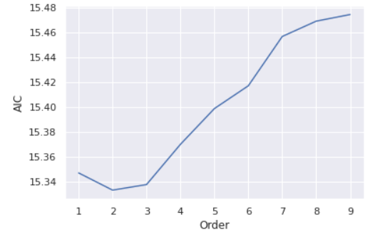

From the plot, the lowest AIC score is achieved at the order of 2 and then the AIC scores show an increasing trend with the order p gets larger. Hence, we select the 2 as the optimal order of the VAR model. Consequently, we fit order 2 to the forecasting model.

从图中可以看到，最低的AIC得分约为2，然后，随着p的增大，AIC得分呈上升趋势。 因此，我们选择2作为VAR模型的最优顺序。 因此，我们将订单2拟合到预测模型。

let's check the summary of the model:

让我们检查一下模型的摘要：

results = forecasting_model.fit(2)results.summary()

The summary output contains much information:

摘要输出包含许多信息：

Forecasting

预测

We use 2 as the optimal order in fitting the VAR model. Thus, we take the final 2 steps in the training data for forecasting the immediate next step (i.e., the first day of the test data).

我们使用2作为拟合VAR模型的最佳顺序。 因此，我们在训练数据中采取最后的2个步骤来预测下一步(即测试数据的第一天)。

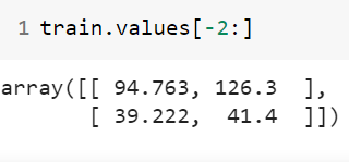
Now, after fitting the model, we forecast for the test data where the last 2 days of training data set as lagged values and steps set as 10 days as we want to forecast for the next 10 days.

现在，在拟合模型之后，我们预测测试数据，其中训练数据的最后2天设置为滞后值，步长设置为10天，因为我们希望在接下来的10天进行预测。

laaged_values = train.values[-2:]forecast = pd.DataFrame(results.forecast(y= laaged_values, steps=10), index = test.index, columns= ['realgdp_1d', 'realdpi_1d'])forecast

The output:

输出：

We have to note that the aforementioned forecasts are for the one differenced model. Hence, we must reverse the first differenced forecasts into the original forecast values.

我们必须注意，上述预测是针对一种差异模型的。 因此，我们必须将最初的差异预测反转为原始预测值。

forecast["realgdp_forecasted"] = data1["realgdp"].iloc[-10-1] +   forecast_1D['realgdp_1d'].cumsum()forecast["realdpi_forecasted"] = data1["realdpi"].iloc[-10-1] +      forecast_1D['realdpi_1d'].cumsum() 

output:

输出：

The first two columns are the forecasted values for 1 differenced series and the last two columns show the forecasted values for the original series.

前两列是1个差异序列的预测值，后两列显示原始序列的预测值。

Now, we visualize the original test values and the forecasted values by VAR.

现在，我们通过VAR可视化原始测试值和预测值。

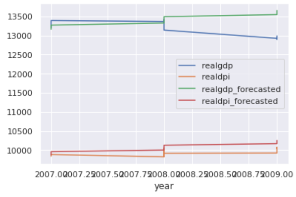
The original realdpi and the forecasted realdpi show a similar pattern throwout the forecasted days. For realgdp: the first half of the forecasted values show a similar pattern as the original values, on the other hand, the last half of the forecasted values do not follow similar pattern.

原始的realdpi和预测的realdpi显示出相似的模式，从而排除了预测的天数。 对于realgdp：预测值的前半部分显示与原始值相似的模式，另一方面，预测值的后半部分没有遵循相似的模式。

To sum up, in this article, we discuss multivariate time series analysis and applied the VAR model on a real-world multivariate time series dataset.

综上所述，在本文​​中，我们讨论了多元时间序列分析，并将VAR模型应用于实际的多元时间序列数据集。

You can also read the article — A real-world time series data analysis and forecasting, where I applied ARIMA (univariate time series analysis model) to forecast univariate time series data.

您还可以阅读这篇文章- 真实的时间序列数据分析和预测 ，在这里我应用了ARIMA(单变量时间序列分析模型)来预测单变量时间序列数据。

[1] https://homepage.univie.ac.at/robert.kunst/prognos4.pdf

[1] https://homepage.univie.ac.at/robert.kunst/prognos4.pdf

[2] https://www.aptech.com/blog/introduction-to-the-fundamentals-of-time-series-data-and-analysis/

[2] https://www.aptech.com/blog/introduction-to-the-fundamentals-of-time-series-data-and-analysis/

[3] https://www.statsmodels.org/stable/index.html

[3] https://www.statsmodels.org/stable/index.html