ARIMA models can be quite adept when it comes to modelling the overall trend of a series along with seasonal patterns.

ARIMA模型可以很好地建模一系列总体趋势以及季节性模式。

In a previous article titled SARIMA: Forecasting Seasonal Data with Python and R, the use of an ARIMA model for forecasting maximum air temperature values for Dublin, Ireland was used.

在上一篇名为SARIMA：使用Python和R预测季节性数据的文章中，使用了ARIMA模型来预测爱尔兰都柏林的最高气温。

The results showed significant accuracy, with 70% of the predictions ranging within 10% of the actual temperature values.

结果显示出显着的准确性，其中70％的预测值在实际温度值的10％范围内。

预测更多极端天气情况 (Forecasting More Extreme Weather Conditions)

That said, the data that was being used for the previous example took temperature values that did not particularly show extreme values. For instance, the minimum temperature value was 4.8°C while the maximum temperature value was 28.7°C. Neither of these values lie outside the norm for typical yearly Irish weather.

就是说，先前示例中使用的数据采用的温度值并未特别显示极端值。 例如，最小温度值为4.8°C，而最大温度值为28.7°C。 这些值都不超出典型的爱尔兰年度天气的标准。

However, let’s consider a more extreme example.

但是，让我们考虑一个更极端的例子。

Braemar is a village located in the Scottish highlands in Aberdeenshire, and is known as one of the coldest places in the United Kingdom in winter. In January 1982, a low of -27.2°C was recorded at this location according to the UK Met Office — which deviates strongly from the average minimum temperature of -1.5°C that was recorded between 1981–2010.

Braemar是位于阿伯丁郡苏格兰高地的一个村庄，被誉为冬季英国最冷的地方之一。 根据英国气象局的数据 ，1982年1月，该地点的最低温度为-27.2°C，这与1981-2010年间记录的平均最低温度 -1.5°C明显不同。

How would an ARIMA model perform when forecasting an abnormally cold winter for Braemar?

预测Braemar异常寒冷的冬天时，ARIMA模型将如何执行？

An ARIMA model is built using monthly Met Office data from January 1959 — July 2020 (contains public sector information licensed under the Open Government Licence v1.0).

ARIMA模型是使用1959年1月至2020年7月的大都会办公室每月数据构建的(包含根据开放政府许可证v1.0 许可的公共部门信息)。

The time series is defined:

时间序列定义为：

weatherarima <- ts(mydata$tmin[1:591], start = c(1959,1), frequency = 12)plot(weatherarima,type="l",ylab="Temperature")title("Minimum Recorded Monthly Temperature: Braemar, Scotland")

Here is a plot of the monthly data:

以下是每月数据的图表：

Here is an overview of the individual time series components:

以下是各个时间序列组成部分的概述：

ARIMA模型配置 (ARIMA Model Configuration)

80% of the dataset (the first 591 months of data) are used to build the ARIMA model. The latter 20% of time series data is then used as validation data to compare the accuracy of the predictions to the actual values.

数据集的80％(最初的591个月的数据)用于构建ARIMA模型。 然后将时间序列数据的后20％用作验证数据，以将预测的准确性与实际值进行比较。

Using auto.arima, the p, d, and q coordinates of best fit are selected:

使用auto.arima，选择最合适的p ， d和q坐标：

# ARIMAfitweatherarima<-auto.arima(weatherarima, trace=TRUE, test="kpss", ic="bic")fitweatherarimaconfint(fitweatherarima)plot(weatherarima,type='l')title('Minimum Recorded Monthly Temperature: Braemar, Scotland')

The best configuration is selected as follows:

最佳配置选择如下：

> # ARIMA> fitweatherarima<-auto.arima(weatherarima, trace=TRUE, test="kpss", ic="bic")Fitting models using approximations to speed things up...ARIMA(2,0,2)(1,1,1)[12] with drift         : 2257.369 ARIMA(0,0,0)(0,1,0)[12] with drift         : 2565.334 ARIMA(1,0,0)(1,1,0)[12] with drift         : 2425.901 ARIMA(0,0,1)(0,1,1)[12] with drift         : 2246.551 ARIMA(0,0,0)(0,1,0)[12]                    : 2558.978 ARIMA(0,0,1)(0,1,0)[12] with drift         : 2558.621 ARIMA(0,0,1)(1,1,1)[12] with drift         : 2242.724 ARIMA(0,0,1)(1,1,0)[12] with drift         : 2427.871 ARIMA(0,0,1)(2,1,1)[12] with drift         : 2259.357 ARIMA(0,0,1)(1,1,2)[12] with drift         : Inf ARIMA(0,0,1)(0,1,2)[12] with drift         : 2252.908 ARIMA(0,0,1)(2,1,0)[12] with drift         : 2341.9 ARIMA(0,0,1)(2,1,2)[12] with drift         : 2249.612 ARIMA(0,0,0)(1,1,1)[12] with drift         : 2264.59 ARIMA(1,0,1)(1,1,1)[12] with drift         : 2248.085 ARIMA(0,0,2)(1,1,1)[12] with drift         : 2246.688 ARIMA(1,0,0)(1,1,1)[12] with drift         : 2241.727 ARIMA(1,0,0)(0,1,1)[12] with drift         : Inf ARIMA(1,0,0)(2,1,1)[12] with drift         : 2261.885 ARIMA(1,0,0)(1,1,2)[12] with drift         : Inf ARIMA(1,0,0)(0,1,0)[12] with drift         : 2556.722 ARIMA(1,0,0)(0,1,2)[12] with drift         : Inf ARIMA(1,0,0)(2,1,0)[12] with drift         : 2338.482 ARIMA(1,0,0)(2,1,2)[12] with drift         : 2248.515 ARIMA(2,0,0)(1,1,1)[12] with drift         : 2250.884 ARIMA(2,0,1)(1,1,1)[12] with drift         : 2254.411 ARIMA(1,0,0)(1,1,1)[12]                    : 2237.953 ARIMA(1,0,0)(0,1,1)[12]                    : Inf ARIMA(1,0,0)(1,1,0)[12]                    : 2419.587 ARIMA(1,0,0)(2,1,1)[12]                    : 2256.396 ARIMA(1,0,0)(1,1,2)[12]                    : Inf ARIMA(1,0,0)(0,1,0)[12]                    : 2550.361 ARIMA(1,0,0)(0,1,2)[12]                    : Inf ARIMA(1,0,0)(2,1,0)[12]                    : 2332.136 ARIMA(1,0,0)(2,1,2)[12]                    : 2243.701 ARIMA(0,0,0)(1,1,1)[12]                    : 2262.382 ARIMA(2,0,0)(1,1,1)[12]                    : 2245.429 ARIMA(1,0,1)(1,1,1)[12]                    : 2244.31 ARIMA(0,0,1)(1,1,1)[12]                    : 2239.268 ARIMA(2,0,1)(1,1,1)[12]                    : 2249.168Now re-fitting the best model(s) without approximations...ARIMA(1,0,0)(1,1,1)[12]                    : Inf ARIMA(0,0,1)(1,1,1)[12]                    : Inf ARIMA(1,0,0)(1,1,1)[12] with drift         : Inf ARIMA(0,0,1)(1,1,1)[12] with drift         : Inf ARIMA(1,0,0)(2,1,2)[12]                    : Inf ARIMA(1,0,1)(1,1,1)[12]                    : Inf ARIMA(2,0,0)(1,1,1)[12]                    : Inf ARIMA(0,0,1)(0,1,1)[12] with drift         : Inf ARIMA(0,0,2)(1,1,1)[12] with drift         : Inf ARIMA(1,0,1)(1,1,1)[12] with drift         : Inf ARIMA(1,0,0)(2,1,2)[12] with drift         : Inf ARIMA(2,0,1)(1,1,1)[12]                    : Inf ARIMA(0,0,1)(2,1,2)[12] with drift         : Inf ARIMA(2,0,0)(1,1,1)[12] with drift         : Inf ARIMA(0,0,1)(0,1,2)[12] with drift         : Inf ARIMA(2,0,1)(1,1,1)[12] with drift         : Inf ARIMA(1,0,0)(2,1,1)[12]                    : Inf ARIMA(2,0,2)(1,1,1)[12] with drift         : Inf ARIMA(0,0,1)(2,1,1)[12] with drift         : Inf ARIMA(1,0,0)(2,1,1)[12] with drift         : Inf ARIMA(0,0,0)(1,1,1)[12]                    : Inf ARIMA(0,0,0)(1,1,1)[12] with drift         : Inf ARIMA(1,0,0)(2,1,0)[12]                    : 2355.279Best model: ARIMA(1,0,0)(2,1,0)[12]

The parameters of the model are as follows:

该模型的参数如下：

> fitweatherarimaSeries: weatherarima ARIMA(1,0,0)(2,1,0)[12]Coefficients:         ar1     sar1     sar2      0.2372  -0.6523  -0.3915s.e.  0.0411   0.0392   0.0393

Using the configured model ARIMA(1,0,0)(2,1,0)[12], the forecasted values are generated:

使用配置的模型ARIMA(1,0,0)(2,1,0)[12] ，将生成预测值：

forecastedvalues=forecast(fitweatherarima,h=148)forecastedvaluesplot(forecastedvalues)

Here is a plot of the forecasts:

这是预测的图：

Now, a data frame can be generated to compare the forecasted with actual values:

现在，可以生成一个数据框以将预测值与实际值进行比较：

df<-data.frame(mydata$tmin[592:739],forecastedvalues$mean)col_headings<-c("Actual Weather","Forecasted Weather")names(df)<-col_headingsattach(df)

Additionally, using the Metrics library in R, the RMSE (root mean squared error) value can be calculated.

此外，使用R中的Metrics库，可以计算RMSE(均方根误差)值。

> library(Metrics)> rmse(df$`Actual Weather`,df$`Forecasted Weather`)[1] 1.780472> mean(df$`Actual Weather`)[1] 2.876351> var(df$`Actual Weather`)[1] 17.15774

It is observed that with a mean temperature of 2.87°C, the recorded RMSE of 1.78 is significantly large when compared to the mean.

可以看出，平均温度为2.87°C，与平均温度相比，记录的RMSE为1.78很大。

Let’s investigate the more extreme values in the data further.

让我们进一步研究数据中更极端的值。

We can see that when it comes to forecasting particularly extreme minimum temperatures (below -4°C for the sake of argument), we see that the ARIMA model significantly overestimates the value of the minimum temperature.

我们可以看到，在预测特别极端的最低温度(出于争论的目的，低于-4°C)时，我们可以看到ARIMA模型大大高估了最低温度的值。

In this regard, the size of the RMSE is just over 60% relative to the mean temperature of 2.87°C in the test set — for the reason that RMSE penalises larger errors more heavily.

在这方面，RMSE的大小相对于测试集中的平均温度2.87°C刚好超过60％，这是因为RMSE会更严厉地惩罚较大的误差。

In this regard, it would seem that the ARIMA model is effective at capturing temperatures that are more in the normal range of values.

在这方面，ARIMA模型似乎可以有效地捕获更多处于正常值范围内的温度。

However, the model falls short in predicting values at the more extreme ends of the scales — particularly for the winter months.

但是，该模型无法预测更极端的数值，尤其是在冬季。

That said, what if the lower end of the ARIMA forecast was used?

就是说，如果使用ARIMA预测的下限怎么办？

df<-data.frame(mydata$tmin[592:739],forecastedvalues$lower)col_headings<-c("Actual Weather","Forecasted Weather")names(df)<-col_headingsattach(df)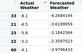

We see that while the model is performing better in forecasting the minimum values, the actual minimums still exceed that of the forecast.

我们看到，尽管模型在预测最小值方面表现更好，但实际最小值仍超过了预测值。

Moreover, this does not solve the problem as it means that the model will now significantly underestimate temperature values above the mean.

此外，这不能解决问题，因为这意味着该模型现在将大大低估高于平均值的温度值。

As a result, the RMSE increases significantly:

结果，RMSE显着增加：

> library(Metrics)> rmse(df$`Actual Weather`,df$`Forecasted Weather`)[1] 3.907014> mean(df$`Actual Weather`)[1] 2.876351

In this regard, ARIMA models should be interpreted with caution. While they can be effective in capturing seasonality and the overall trend, they can fall short in forecasting values that fall significantly outside the norm.

在这方面，ARIMA模型应谨慎解释。 尽管它们可以有效地捕获季节性和总体趋势，但在预测值超出正常范围的情况下可能会不足。

When it comes to forecasting such values, statistical tools such as Monte Carlo simulations can be more effective in modelling a potential range of more extreme values. Here is a follow-up article that discusses how extreme weather events can potentially be modelled using this method.

在预测此类值时，诸如蒙特卡洛模拟之类的统计工具可以更有效地建模更极端值的潜在范围。 以下是后续文章 ，讨论了如何使用这种方法来模拟极端天气事件。

结论 (Conclusion)

In this example, we have seen that ARIMA can be limited in forecasting extreme values. While the model is adept at modelling seasonality and trends, outliers are difficult to forecast for ARIMA for the very reason that they lie outside of the general trend as captured by the model.

在此示例中，我们已经看到ARIMA在预测极值时可能受到限制。 尽管该模型擅长于对季节和趋势进行建模，但由于ARIMA超出了模型捕获的总体趋势，因此很难预测ARIMA。

Many thanks for reading, and you can find more of my data science content at michael-grogan.com.

非常感谢您的阅读，您可以在michael-grogan.com上找到更多我的数据科学内容。

Disclaimer: This article is written on an “as is” basis and without warranty. It was written with the intention of providing an overview of data science concepts, and should not be interpreted as professional advice in any way. The findings and interpretations in this article are those of the author and are not endorsed by or affiliated with the UK Met Office in any way.

免责声明：本文按“原样”撰写，不作任何担保。 它旨在提供数据科学概念的概述，并且不应以任何方式解释为专业建议。 本文中的发现和解释仅归作者所有，并不以任何方式得到英国气象局的认可或附属。