接近组数据(组间) (Approaching group data (between-group))

A typical situation regarding solving an experimental question using a data-driven approach involves several groups that differ in (hopefully) one, sometimes more variables.

使用数据驱动的方法解决实验性问题的典型情况涉及几个组(希望)不同，有时甚至更多。

Say you collect data on people that either ate (Group 1) or did not eat chocolate (Group 2). Because you know the literature very well, and you are an expert in your field, you believe that people that ate chocolate are more likely to ride camels than people that did not eat the chocolate.

假设您收集的是吃过(第1组)或没有吃巧克力(第2组)的人的数据。 因为您非常了解文献，并且您是该领域的专家，所以您认为吃巧克力的人比没有吃巧克力的人骑骆驼的可能性更高。

You now want to prove that empirically.

您现在想凭经验证明这一点。

I will be generating simulation data using Python, to demonstrate how permutation testing can be a great tool to detect within group variations that could reveal peculiar patterns of some individuals. If your two groups are statistically different, then you might explore what underlying parameters could account for this difference. If your two groups are not different, you might want to explore whether some data points still behave “weirdly”, to decide whether to keep on collecting data or dropping the topic.

我将使用Python生成仿真数据，以演示置换测试如何成为检测组内变异的好工具，这些变异可以揭示某些个体的特殊模式。 如果两组在统计上不同，那么您可能会探索哪些基础参数可以解释这一差异。 如果两组没有不同，则可能要探索某些数据点是否仍然表现“怪异”，以决定是继续收集数据还是删除主题。

# Load standard librariesimport panda as pd import numpy as npimport matplotlib.pyplot as plt

Now one typical approach in this (a bit crazy) experimental situation would be to look at the difference in camel riding propensity in each group. You could compute the proportions of camel riding actions, or the time spent on a camel, or any other dependent variable that might capture the effect you believe to be true.

现在，在这种(有点疯狂)实验情况下，一种典型的方法是查看每组中骑骆驼倾向的差异。 您可以计算骑骆驼动作的比例，骑骆驼的时间或其他任何可能捕捉到您认为是真实的效果的因变量。

产生资料 (Generating data)

Let’s generate the distribution of the chocolate group:

让我们生成巧克力组的分布：

# Set seed for replicabilitynp.random.seed(42)# Set Mean, SD and sample sizemean = 10; sd=1; sample_size=1000# Generate distribution according to parameterschocolate_distibution = np.random.normal(loc=mean, scale=sd, ssize=sample_size)# Show dataplt.hist(chocolate_distibution)plt.ylabel("Time spent on a camel")plt.title("Chocolate Group")

As you can see, I created a distribution centered around 10mn. Now let’s create the second distribution, which could be the control, centered at 9mn.

如您所见，我创建了一个以1000万为中心的发行版。 现在，让我们创建第二个分布，该分布可能是控件，以900万为中心。

mean = 9; sd=1; sample_size=1000non_chocolate_distibution = np.random.normal(loc=mean, scale=sd, size=sample_size)fig = plt.figure()plt.hist(non_chocolate_distibution)plt.ylabel("Time spent on a camel")plt.title("Non Chocolate Group")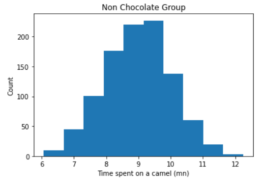

OK! So now we have our two simulated distributions, and we made sure that they differed in their mean. With the sample size we used, we can be quite sure we would have two significantly different populations here, but let’s make sure of that. Let’s quickly visualize that:

好！ 因此，现在我们有了两个模拟分布，并确保它们的均值不同。 使用我们使用的样本量，我们可以确定这里会有两个明显不同的总体，但是让我们确定一下。 让我们快速想象一下：

We can use an independent sample t-test to get an idea of how different these distributions might be. Note that since the distributions are normally distributed (you can test that with a Shapiro or KS test), and the sample size is very high, parametric testing (under which t-test falls) is permitted. We should run a Levene’s test as well to check the homogeneity of variances, but for the sake of argumentation, let’s move on.

我们可以使用独立的样本t检验来了解这些分布可能有多大差异。 请注意，由于分布是正态分布的(可以使用Shapiro或KS检验进行测试)，并且样本量非常大，因此可以进行参数检验(t检验属于这种检验)。 我们也应该运行Levene检验来检验方差的均匀性，但是为了论证，让我们继续。

from scipy import statst, p = stats.ttest_ind(a=chocolate_distibution, b=non_chocolate_distibution, axis=0, equal_var=True)print('t-value = ' + str(t))print('p-value = ' + str(p))

Good, that worked as expected. Note that given the sample size, you are able to detect even very small effects, such as this one (distributions’ means differ only by 1mn).

很好，按预期工作。 请注意，在给定样本量的情况下，您甚至可以检测到很小的影响，例如这种影响(分布的均值相差仅100万)。

If these would be real distributions, one would have some evidence that chocolate affects the time spent riding a camel (and should of course dig down a bit more to see what could explain that strange effect…).

如果这些是真实的分布，则将有一些证据表明巧克力会影响骑骆驼的时间(当然，应该多挖一点，看看有什么能解释这种奇怪的作用……)。

I should note that at some point tough, this kind of statistics become dangerous because of the high sample size, that outputs extremely high p-values for even low effects. I discuss a bit this issue in this post. Anyway, this post is about approaching individual data, so let’s move on.

我应该指出，由于样本量太大，这种统计数据有时会变得很危险，因为即使样本量很小，其输出的p值也非常高。 我在这篇文章中讨论了这个问题。 无论如何，这篇文章是关于处理单个数据的，所以让我们继续。

处理单个数据(组内) (Approaching individual data (within-group))

Now let’s assume that for each of these participants, you recorded multiple choices (Yes or No) to ride a camel (you probably want to do this a few times per participants to get reliable data). Thus, you have repeated measures, at different time points. You know that your groups are significantly different, but what about `within group` variance? And what about an alternative scenario where your groups don’t differ, but you know some individuals showed very particular behavior? The method of permutation can be used in both cases, but let’s use the scenario generated above where groups are significanly different.

现在，假设对于每个参与者，您记录了骑骆驼的多个选择(是或否)(您可能希望每个参与者进行几次此操作以获得可靠的数据)。 因此，您将在不同的时间点重复进行测量。 您知道您的小组有很大不同，但是“小组内”差异又如何呢？ 在您的小组没有不同但您知道某些人表现出非常特殊的行为的情况下，又该如何呢？ 两种情况下都可以使用置换方法，但是让我们使用上面生成的方案，其中组明显不同。

What you might observe is that, while at the group level you do have a increased tendency to ride camels after your manipulation (eg, giving sweet sweet chocolate to your subjects), within the chocolate group, some people have a very high tendency while others are actually no different than the No Chocolate group. Vice versa, maybe within the non chocolate group, while the majority did not show an increase in the variable, some did (but that effect is diluted by the group’s tendency).

您可能会观察到的是，虽然在小组级别上，您在操纵后确实骑骆驼的趋势有所增加(例如，给受试者提供甜甜的巧克力)，但是在巧克力小组中 ，有些人的趋势非常高，而其他人实际上与“无巧克力”组没有什么不同。 反之亦然，也许在非巧克力组中，虽然大多数没有显示变量的增加，但有一些确实存在(但这种影响因该组的趋势而被淡化)。

One way to test that would be to use a permutation test, to test each participants against its own choice patterns.

一种测试方法是使用置换测试，以针对每个参与者自己的选择模式进行测试。

资料背景 (Data background)

Since we are talking about choices, we are looking at a binomial distribution, where say 1 = Decision to ride a camel and 0 = Decision not to ride a camel.Let’s generate such a distribution for a given participant that would make 100 decisions:

既然我们在谈论选择，我们正在看一个二项式分布，其中说1 =骑骆驼的决定和0 = 不骑骆驼的决定，让我们为给定的参与者生成这样的分布，它将做出100个决定：

Below, one example where I generate the data for one person, and bias it so that I get a higher number of ones than zeros (that would be the kind of behavior expected by a participant in the chocolate group

在下面的示例中，我为一个人生成数据，并对数据进行偏倚，这样我得到的数据要多于零(这是巧克力组参与者期望的行为)

distr = np.random.binomial(1, 0.7, size=100)print(distr)

# Plot the cumulative datapd.Series(distr).plot(kind=’hist’)

We can clearly see that we have more ones than zeros, as wished.

我们可以清楚地看到，正如我们所希望的那样，我们的数字多于零。

Let’s generate such choice patterns for different participants in each group.

让我们为每个组中的不同参与者生成这种选择模式。

为所有参与者生成选择数据 (Generating choice data for all participants)

Let’s say that each group will be composed of 20 participants that made 100 choices.

假设每个小组将由20个参与者组成，他们做出了100个选择。

In an experimental setting, we should probably have measured the initial preference of each participant to like camel riding (maybe some people, for some reason, like it more than others, and that should be corrected for). That measure can be used as baseline, to account for initial differences in camel riding for each participant (that, if not measured, could explain differences later on).

在实验环境中，我们可能应该已经测量了每个参与者对骑骆驼的喜好(也许某些人由于某种原因比其他人更喜欢骆驼，应该对此进行纠正)。 该度量可以用作基准，以说明每个参与者骑骆驼的初始差异(如果不进行度量，则可以稍后解释差异)。

We thus will generate a baseline phase (before giving them chocolate) and an experimental phase (after giving them chocolate in the chocolate group, and say another neutral substance in the non chocolate group (as a control manipulation).

因此，我们将生成一个基线阶段(在给他们巧克力之前)和一个实验阶段(在给他们巧克力组中的巧克力之后，并说非巧克力组中的另一种中性物质(作为对照操作)。

A few points:1) I will generate biased distributions that follow the pattern found before, i.e., that people that ate chocolate are more likely to ride a camel.2) I will produce baseline choice levels similar between the two groups, to make the between group comparison statistically valid. That is important and should be checked before you run more tests, since your groups should be as comparable as possible.3) I will include in each of these groups a few participants that behave according to the pattern in the other group, so that we can use a permutation method to detect these guys.

有几点要点： 1)我将按照以前发现的模式生成有偏差的分布，即吃巧克力的人骑骆驼的可能性更大。 2)我将产生两组之间相似的基线选择水平，以使组之间的比较在统计上有效。 这很重要，应该在运行更多测试之前进行检查，因为您的组应尽可能具有可比性。 3)我将在每个小组中包括一些参与者，这些参与者根据另一小组中的模式进行举止，以便我们可以使用排列方法来检测这些家伙。

Below, the function I wrote to generate this simulation data.

下面是我编写的用于生成此模拟数据的函数。

def generate_simulation_data(nParticipants, nChoicesBase,             nChoicesExp, binomial_ratio):    """    Generates a simulation choice distribution based on parameters    Function uses a binomial distribution as basis    params: (int) nParticipants, number of participants for which   we need data    params: (int) nChoicesBase, number of choices made in the baseline period    params: (int) nChoicesExp, number of choices made in the experimental period    params: (list) binomial_ratio, ratio of 1&0 in the resulting binomial distribution. Best is to propose a list of several values of obtain variability.    """    # Pre Allocate    group = pd.DataFrame()    # Loop over participants. For each draw a binonimal choice distribution    for i in range (0,nParticipants):        # Compute choices to ride a camel before drinking, same for both groups (0.5)         choices_before = np.random.binomial(1, 0.4, size=nChoicesBase)         # Compute choices to ride a camel after drinking, different per group (defined by binomial ratio)        # generate distribution        choices_after  = np.random.binomial(1, np.random.choice(binomial_ratio,replace=True), size=nChoicesExp)        # Concatenate        choices = np.concatenate([choices_before, choices_after])        # Store in dataframe        group.loc[:,i] = choices    return group.T

Let’s generate choice data for the chocolate group, with the parameters we defined earlier. I use binomial ratios starting at 0.5 to create a few indifferent individuals within this group. I also use ratios > 0.5 since this group should still contain individuals with high preference levels.

让我们使用前面定义的参数生成巧克力组的选择数据。 我使用从0.5开始的二项式比率在该组中创建了一些无关紧要的人。 我也使用比率> 0.5，因为该组仍应包含具有较高优先级的个人。

chocolate_grp = generate_simulation_data(nParticipants=20,              nChoicesBase=20, nChoicesExp=100, binomial_ratio=[0.5,0.6,0.7,0.8,0.9])

As we can see, we generated binary choice data for 120 participants. The screenshot shows part of these choices for some participants (row index).

如我们所见，我们为120名参与者生成了二元选择数据。 屏幕截图显示了一些参与者的部分选择(行索引)。

We can now quickly plot the summed choices for riding a camel for each of these participants to verify that indeed, we have a few indifferent ones (data points around 50), but most of them have a preference, more or less pronounced, to ride a camel.

现在，我们可以为每个参与者快速绘制骑骆驼的总和选择，以验证确实有一些冷漠的人(数据点大约为50)，但是其中大多数人或多或少都倾向于骑车一头骆驼。

def plot_group_hist(data, title):    data.sum(axis=1).plot(kind='hist')    plt.ylabel("Number of participants")    plt.xlabel("Repeated choices to ride a camel")    plt.title(title)plot_group_hist(chocolate_grp, title=' Chocolate group')

Instead of simply summing up the choices to ride a camel, let’s compute a single value per participant that would reflect their preference or aversion to camel ride.

与其简单地总结骑骆驼的选择，不如计算每个参与者的单个值，以反映他们对骆驼骑的偏好或反感。

I will be using the following equation, that basically computes a score between [-1;+1], +1 reflecting a complete switch for camel ride preference after drinking, and vice versa. This is equivalent to other normalizations (or standardizations) that you can find in SciKit Learn for instance.

我将使用以下等式，该等式基本上计算出[-1; +1]，+ 1之间的得分，这反映了饮酒后骆驼骑行偏好的完全转换，反之亦然。 例如，这等同于您可以在SciKit Learn中找到的其他标准化(或标准化)。

Now, let’s use that equation to compute, for each participant, a score that would inform on the propensity to ride a camel. I use the function depicted below.

现在，让我们使用该方程式为每个参与者计算一个分数，该分数将说明骑骆驼的倾向。 我使用下面描述的功能。

def indiv_score(data):    """    Calculate a normalized score for each participant    Baseline phase is taken for the first 20 decisions    Trials 21 to 60 are used as actual experimental choices    """    # Baseline is the first 20 choices, experimental is from choice 21 onwards    score = ((data.loc[20:60].mean() - data.loc[0:19].mean())        / (data.loc[20:60].mean() + data.loc[0:19].mean())        )    return scoredef compute_indiv_score(data):    """    Compute score for all individuals in the dataset    """    # Pre Allocate    score = pd.DataFrame(columns = ['score'])    # Loop over individuals to calculate score for each one    for i in range(0,len(data)):        # Calculate score        curr_score = indiv_score(data.loc[i,:])        # Store score        score.loc[i,'score'] = curr_score    return scorescore_chocolate = compute_indiv_score(chocolate_grp)score_chocolate.plot(kind='hist')

We can interpret these scores as suggesting that some individuals showed >50% higher preference to ride a camel after drinking chocolate, while the majority showed an increase in preference of approximately 20/40%. Note how a few individuals, although pertaining to this group, show an almost opposite pattern.

我们可以将这些分数解释为，表明一些人在喝完巧克力后对骑骆驼的偏好提高了50％以上，而大多数人的偏好提高了约20/40％。 请注意，尽管有些人属于这个群体，却表现出几乎相反的模式。

Now let’s generate and look at data for the control, non chocolate group

现在让我们生成并查看非巧克力对照组的数据

plot_group_hist(non_chocolate_grp, title='Non chocolate group')\

We can already see that the number of choices to ride a camel are quite low compared to the chocolate group plot.

我们已经可以看到，与巧克力集团相比，骑骆驼的选择数量非常少。

OK! Now we have our participants. Let’s run a permutation test to detect which participants were significantly preferring riding a camel in each group. Based on the between group statistics, we expect that number to be higher in the chocolate than in the non chocolate group.

好！ 现在我们有我们的参与者。 让我们运行一个置换测试，以检测哪些参与者在每个组中明显更喜欢骑骆驼。 根据小组之间的统计，我们预计巧克力中的这一数字将高于非巧克力组。

排列测试 (Permutation test)

A permutation test consists in shuffling the data, within each participant, to create a new distribution of data that would reflect a virtual, but given the data possible, distribution. That operation is performed many times to generate a virtual distribution against which the actual true data is compared to.

排列测试包括在每个参与者内对数据进行混排，以创建新的数据分布，该分布将反映虚拟但有可能的数据分布。 多次执行该操作以生成虚拟分布，将其与实际的真实数据进行比较。

In our case, we will shuffle the data of each participant between the initial measurement (baseline likelihood to ride a camel) and the post measurement phase (same measure after drinking, in each group).

在我们的案例中，我们将在初始测量(骑骆驼的基准可能性)和测量后阶段(每组喝酒后的相同测量)之间对每个参与者的数据进行混洗。

The function below runs a permutation test for all participants in a given group.For each participant, it shuffles the choice data nReps times, and calculate a confidence interval (you can define whether you want it one or two sided) and checks the location of the real choice data related to this CI. When outside of it, the participant is said to have a significant preference for camel riding.

下面的函数对给定组中的所有参与者进行排列测试，对于每个参与者，其洗净选择数据nReps次，并计算置信区间(您可以定义是单面还是双面)并检查位置与此CI相关的实际选择数据。 在外面时，据说参与者特别喜欢骑骆驼。

I provide the function to run the permutation below. If is a bit long, but it does the job ;)

我提供了运行以下排列的功能。 如果有点长，但是可以完成工作；)

def run_permutation(data, direct='two-sided', nReps=1000, print_output=False):    """    Run a permutation test.    For each permutation, a score is calculated and store in an array.    Once all permutations are performed for that given participants, the function computes the real score    It then compares the real score with the confidence interval.

    The ouput is a datafram containing all important statistical information.    params: (df) data, dataframe with choice data    params: (str) direct, default 'two-sided'. Set to 'one-sided' to compute a one sided confidence interval    params: (int) nReps. number of iterations     params: (boolean), default=False. True if feedback to user is needed    """    # PreAllocate significance    output=pd.DataFrame(columns=['Participant', 'Real_Score', 'Lower_CI', 'Upper_CI', 'Significance'])for iParticipant in range(0,data.shape[0]):        # Pre Allocate        scores = pd.Series('float')        # Start repetition Loop        if print_output == True:            print('Participant #' +str(iParticipant))        output.loc[iParticipant, 'Participant'] = iParticipant        for iRep in range(0,nReps):            # Store initial choice distribution to compute real true score            initial_dat = data.loc[iParticipant,:]            # Create a copy            curr_dat = initial_dat.copy()            # Shuffle data            np.random.shuffle(curr_dat)            # Calculate score with shuffled data            scores[iRep] = indiv_score(curr_dat)

        # Sort scores to compute confidence interval        scores = scores.sort_values().reset_index(drop=True)        # Calculate confidence interval bounds, based on directed hypothesis        if direct == 'two-sided':            upper = scores.iloc[np.ceil(scores.shape[0]*0.95).astype(int)]            lower = scores.iloc[np.ceil(scores.shape[0]*0.05).astype(int)]        elif direct == 'one-sided':            upper = scores.iloc[np.ceil(scores.shape[0]*0.975).astype(int)]            lower = scores.iloc[np.ceil(scores.shape[0]*0.025).astype(int)]output.loc[iParticipant, 'Lower_CI'] = lower        output.loc[iParticipant, 'Upper_CI'] = upper        if print_output == True:            print ('CI = [' +str(np.round(lower,decimals=2)) + ' ; ' + str(np.round(upper,decimals=2)) + ']')        # Calculate real score        real_score = indiv_score(initial_dat)        output.loc[iParticipant, 'Real_Score'] = real_score        if print_output == True:            print('Real score = ' + str(np.round(real_score,decimals=2)))        # Check whether score is outside CI bound        if (real_score < upper) & (real_score > lower):            output.loc[iParticipant, 'Significance'] =0            if print_output == True:                print('Not Significant')        elif real_score >= upper:            output.loc[iParticipant, 'Significance'] =1            if print_output == True:                print('Significantly above')        else: output.loc[iParticipant, 'Significance']  = -1; print('Significantly below')        if print_output == True:            print('')    return output

Now let’s run the permutation test, and look at individual score values

现在让我们运行置换测试，并查看各个得分值

output_chocolate = run_permutation(chocolate_grp, direct=’two-sided’, nReps=100, print_output=False)output_chocolate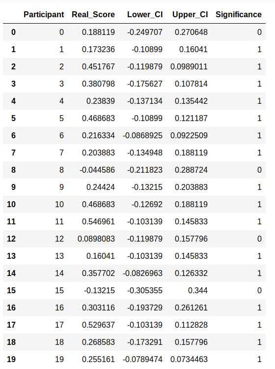

output_non_chocolate = run_permutation(non_chocolate_grp, direct='two-sided', nReps=100, print_output=False)output_non_chocolate

We can see that, as expected from the way we compute the distributions ,we have much more participants that significantly increased their camel ride preference after the baseline measurement in the chocolate group.

我们可以看到，正如我们从计算分布的方式所预期的那样，在巧克力组进行基线测量之后，有更多的参与者显着提高了他们的骆驼骑行偏好。

That is much less likely in the non chocolate group, where we even have one significant decrease in preference (participant #11)

在非巧克力组中，这的可能性要小得多，在该组中，我们的偏好甚至大大降低了(参与者＃11)

We can also see something I find quite important: some participants have a high score but no significant preference, while others have a lower score and a significant preference (see participants 0 & 1 in the chocolate group). That is due to the confidence interval, which is calculated based on each participant’s behavior. Therefore, based on the choice patterns, a given score might fall inside the CI and not be significant, while another, maybe lower score, maybe fall outside this other individual-based CI.

我们还可以看到一些我认为非常重要的东西：一些参与者的得分较高，但没有明显的偏好，而另一些参与者的得分较低，并且有明显的偏好(请参阅巧克力组中的参与者0和1)。 这是由于置信区间是基于每个参与者的行为计算的。 因此，根据选择模式，给定的得分可能落在CI内，并且不显着，而另一个得分可能更低，或者落在其他基于个人的CI之外。

最后的话 (Final words)

That was it. Once this analysis is done, you could look at what other, **unrelated** variables, might differ between the two groups and potentially explain part of the variance in the statistics. This is an approach I used in this publication, and it turned out to be quite useful :)I hope that you found this tutorial helpful.Don’t hesitate to contact me if you have any questions or comments!

就是这样 完成此分析后，您可以查看两组之间** 无关的 **变量可能不同，并可能解释统计数据中的部分方差。 这是我在本出版物中使用的一种方法，结果非常有用:)我希望您对本教程有所帮助。如有任何疑问或意见，请随时与我联系！

Data and notebooks are in this repo: https://github.com/juls-dotcom/permutation

数据和笔记本在此仓库中： https : //github.com/juls-dotcom/permutation