内部AI (Inside AI)

In the world of data, we all love Gaussian distribution (also known as a normal distribution). In real-life, seldom we have normal distribution data. It is skewed, missing data points or has outliers.

在数据世界中，我们都喜欢高斯分布(也称为正态分布)。 在现实生活中，很少有正态分布数据。 它歪斜，缺少数据点或有异常值。

As I mentioned in my earlier article, the strength of Scikit-learn inadvertently works to its disadvantage. Machine learning developers esp. with relatively lesser experience implements an inappropriate algorithm for prediction without grasping particular algorithms salient feature and limitations. We have seen earlier the reason we should not use the decision tree regression algorithm in making a prediction involving extrapolating the data.

正如我在前一篇文章中提到的那样 ，Scikit-learn的优势在无意中起到了不利的作用。 机器学习开发人员，尤其是。 经验相对较少的人在不掌握特定算法的显着特征和局限性的情况下，实施了不合适的预测算法。 前面我们已经看到了在进行涉及外推数据的预测时不应使用决策树回归算法的原因。

The success of any machine learning modelling always starts with understanding the existing dataset on which model will be trained. It is imperative to understand the data well before starting any modelling. I will even go to an extent to say that the prediction accuracy of the model is directly proportional to the extent we know the data.

任何机器学习建模的成功总是始于了解将在其上训练模型的现有数据集。 必须在开始任何建模之前充分了解数据。 我什至会在某种程度上说模型的预测准确性与我们知道数据的程度成正比。

Objective

目的

In this article, we will see the effect of outliers on various regression algorithms available in Scikit-learn, and learn about the most appropriate regression algorithm to apply in such a situation. We will start with a few techniques to understand the data and then train a few of the Sklearn algorithms with the data. Finally, we will compare the training results of the algorithms and learn the potential best algorithms to apply in the case of outliers.

在本文中，我们将看到异常值对Scikit-learn中可用的各种回归算法的影响，并了解适用于这种情况的最合适的回归算法。 我们将从几种了解数据的技术入手，然后根据数据训练一些Sklearn算法。 最后，我们将比较算法的训练结果，并学习适用于异常值的潜在最佳算法。

Training Dataset

训练数据集

The training data consists of 200,000 records of 3 features (independent variable) and 1 target value (dependent variable). The true coefficient of the features 1, feature 2 and feature 3 is 77.74, 23.34, and 7.63 respectively.

训练数据包含200,000条具有3个特征(独立变量)和1个目标值(独立变量)的记录。 特征1，特征2和特征3的真实系数分别为77.74、23.34和7.63。

Step 1- First, we will import the packages required for data analysis and regressions.

步骤1- 首先，w e将导入数据分析和回归所需的软件包。

We will be comparing HuberRegressor, LinearRegression, Ridge, SGDRegressor, ElasticNet, PassiveAggressiveRegressor and Linear Support Vector Regression (SVR), hence we will import the respective packages.

我们将比较HuberRegressor，LinearRegression，Ridge，SGDRegressor，ElasticNet，PassiveAggressiveRegressor和Linear Support Vector Regression(SVR)，因此将分别导入软件包。

Most of the time, few data points are missing in the training data. In that case, if any particular features have a high proportion of null values then it may be better not consider that feature. Else, if a few data points are missing for a feature then either can drop those particular records from training data, or we can replace those missing values with mean, median or constant values. We will import SimpleImputer to fill the missing values.

大多数时候，训练数据中很少有数据点缺失。 在那种情况下，如果任何特定功能具有高比例的空值，则最好不要考虑该功能。 否则，如果某个功能缺少一些数据点，则可以从训练数据中删除那些特定的记录，或者我们可以将这些丢失的值替换为均值，中值或常数。 我们将导入SimpleImputer来填充缺少的值。

We will import the Variance Inflation Factor to find the severity of multicollinearity among the features. We will need Matplotlib and seaborn to draw various plots for analysis.

我们将导入方差通货膨胀因子以找到特征之间多重共线性的严重性。 我们将需要Matplotlib和seaborn绘制各种图进行分析。

from sklearn.linear_model import HuberRegressor,LinearRegression ,Ridge,SGDRegressor,ElasticNet,PassiveAggressiveRegressorfrom sklearn.svm import LinearSVRimport pandas as pdfrom sklearn.impute import SimpleImputerfrom statsmodels.stats.outliers_influence import variance_inflation_factorimport numpy as npimport matplotlib.pyplot as pltimport seaborn as sns

Step 2- In the code below, training data containing 200.000 records are read from excel file into the PandasDataframe called “RawData”. Independent variables are saved into a new DataFrame.

步骤2-在下面的代码中，将包含200.000条记录的训练数据从excel文件中读取到名为“ RawData”的PandasDataframe中。 自变量保存到新的DataFrame中。

RawData=pd.read_excel("Outlier Regression.xlsx")Data=RawData.drop(["Target"], axis=1)

Step 3-Now we will start by getting a sense of the training data and understanding it. In my opinion, a heatmap is a good option to understand the relationship between different features.

步骤3-现在，我们将首先了解并理解训练数据。 我认为，热图是了解不同功能之间关系的一个不错的选择。

sns.heatmap(Data.corr(), cmap="YlGnBu", annot=True)plt.show()

It shows that none of the independent variables (features) is closely related to each other. In case you would like to learn more on the approach and selection criteria of independent variables for regression algorithms, then please read my earlier article on it.

它表明没有一个自变量(特征)彼此密切相关。 如果您想了解更多有关回归算法自变量的方法和选择标准的信息，请阅读我以前的文章。

How to identify the right independent variables for Machine Learning Supervised Algorithms?

如何为机器学习监督算法识别正确的自变量？

Step 4- After getting a sense of the correlation among the features in the training data next we will look into the minimum, maximum, median etc. of each feature value range. This will help us to ascertain whether there are any outliers in the training data and the extent of it. Below code instructs to draw boxplots for all the features.

步骤4-在了解了训练数据中各特征之间的相关性之后，我们将研究每个特征值范围的最小值，最大值，中位数等。 这将有助于我们确定训练数据中是否存在异常值及其范围。 以下代码指示绘制所有功能的箱线图。

sns.boxplot(data=Data, orient="h",palette="Set2")plt.show()

In case you don’t know to read the box plot then please refer the Wikipedia to learn more on it. Feature values are spread across a wide range with a big difference from the median value. This confirms the presence of outlier values in the training dataset.

如果您不知道阅读箱形图，请参考Wikipedia以了解更多信息。 特征值分布在很大范围内，与中值有很大差异。 这确认了训练数据集中存在异常值。

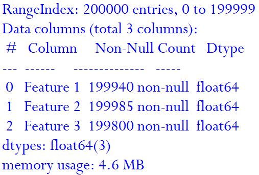
Step 5- We will check if there are any null values in the training data and take any action required before going anywhere near modelling.

第5步-我们将检查训练数据中是否有任何空值，并采取任何必要的措施，然后再进行建模。

print (Data.info())

Here we can see that there are total 200,000 records in the training data and all three features have few values missing. For example, feature 1 has 60 values (200000 –199940) missing.

在这里我们可以看到训练数据中总共有200,000条记录，并且所有三个功能都缺少几个值。 例如，特征1缺少60个值(200000 –199940)。

Step 6- We use SimpleImputer to fill the missing values with the mean values of the other records for a feature. In the below code, we use the strategy= “mean” for the same. Scikit-learn provides different strategies viz. mean, median, most frequent and constant value to replace the missing value. I will suggest you please self explore the effect of each strategy on the training model as a learning exercise.

第6步-我们使用SimpleImputer用功能的其他记录的平均值填充缺失值。 在下面的代码中，我们同样使用strategy =“ mean”。 Scikit-learn提供了不同的策略。 平均，中位数，最频繁和恒定的值来代替缺失值。 我建议您作为学习练习，自我探索每种策略对训练模型的影响。

In the code below, we have created an instance of SimpleImputer with strategy “Mean” and then fit the training data into it to calculate the mean of each feature. Transform method is used to fill the missing values with the mean value.

在下面的代码中，我们创建了一个策略为“ Mean”的SimpleImputer实例，然后将训练数据拟合到其中以计算每个特征的均值。 变换方法用于用平均值填充缺失值。

imputer = SimpleImputer(strategy="mean")imputer.fit(Data)TransformData = imputer.transform(Data)X=pd.DataFrame(TransformData, columns=Data.columns)

Step 7- It is good practice to check the features once more after replacing the missing values to ensure we do not have any null (blank) values remaining in our training dataset.

第7步-好的做法是在替换缺失值之后再次检查特征，以确保我们的训练数据集中没有剩余的任何空(空白)值。

print (X.info())

We can see that now all the features have non-null i.e non-blank values for 200,000 records.

我们可以看到，现在所有功能都具有非空值，即200,000条记录的非空白值。

Step 8- Before we start training the algorithms, let us check the Variance inflation factor (VIF) among the independent variables. VIF quantifies the severity of multicollinearity in an ordinary least squares regression analysis. It provides an index that measures how much the variance (the square of the estimate’s standard deviation) of an estimated regression coefficient is increased because of collinearity. I will encourage you all to read the Wikipedia page on Variance inflation factor to gain a good understanding of it.

步骤8-在开始训练算法之前，让我们检查自变量之间的方差膨胀因子 ( VIF )。 VIF在普通最小二乘回归分析中量化多重共线性的严重性。 它提供了一个指标，用于衡量由于共线性而导致估计的回归系数的方差(估计的标准偏差的平方)增加了多少。 我鼓励大家阅读Wikipedia页面上关于方差膨胀因子的知识 ，以更好地理解它。

vif = pd.DataFrame()vif["features"] = X.columnsvif["vif_Factor"] = [variance_inflation_factor(X.values, i) for i in range(X.shape[1])]print(vif)

In the above code, we calculate the VIF of each independent variables and print it. In general, we should aim for the VIF of less than 10 for the independent variables. We have seen earlier in the heatmap that none of the variables is highly correlated, and the same is reflecting in the VIF index among the features.

在上面的代码中，我们计算每个独立变量的VIF并将其打印出来。 通常，我们应将自变量的VIF设置为小于10。 我们早先在热图中看到，变量没有高度相关，并且在功能之间的VIF索引中也反映出同样的情况。

Step 9- We will extract the target i.e. dependent variable values from the RawData dataframe and save it in a data series.

第9步-我们将从RawData数据帧中提取目标(即因变量值)并将其保存在数据系列中。

y=RawData["Target"].copy()

Step 10- We will be evaluating the performance of various regressors viz. HuberRegressor, LinearRegression, Ridge and others on outlier dataset. In the below code, we created instances of the various regressors.

步骤10-我们将评估各种回归器的性能。 离群数据集上的HuberRegressor，LinearRegression，Ridge等。 在下面的代码中，我们创建了各种回归变量的实例。

Huber = HuberRegressor()Linear = LinearRegression()SGD= SGDRegressor()Ridge=Ridge()SVR=LinearSVR()Elastic=ElasticNet(random_state=0)PassiveAggressiveRegressor= PassiveAggressiveRegressor()

Step 11- We declared a list with instances of the regressions to pass it in sequence in a for a loop later.

第11步-我们声明了一个带有回归实例的列表，以便稍后在循环中依次传递它。

estimators = [Linear,SGD,SVR,Huber, Ridge, Elastic,PassiveAggressiveRegressor]

Step 12- Finally, we will train the models in sequence with the training data set and print the coefficients of the features calculated by the model.

第12步-最后，我们将使用训练数据集按顺序训练模型，并打印由模型计算出的特征的系数。

for i in estimators:    reg= i.fit(X,y)    print(str(i)+" Coefficients:", np.round(i.coef_,2))    print("**************************")

We can observe a wide range of coefficients calculated by different models based on their optimisation and regularisation factors. Feature 1 coefficient calculated coefficient varies from 29.31 to 76.88.

我们可以观察到基于不同模型的优化和正则化因子计算出的各种系数。 特征1系数计算的系数从29.31到76.88。

Due to a few outliers in the training dataset a few models, like linear and ridge regression predicted coefficients nowhere near the true coefficients. Huber regressor is quite robust to the outliers ensuring loss function is not heavily influenced by the outliers while not completely ignoring their effects like TheilSenRegressor and RANSAC Regressor. Linear SVR also more options in the selection of penalties and loss functions and performed better than other models.

由于训练数据集中存在一些离群值，因此一些模型(例如线性和岭回归)预测的系数远不及真实系数。 Huber回归器对异常值非常强大，可以确保损失函数不受异常值的严重影响，同时又不完全忽略其影响，例如TheilSenRegressor和RANSAC回归器。 线性SVR在罚分和损失函数的选择上也有更多选择，并且比其他模型表现更好。

Learning Action for you- We trained different models with a training data set containing outliers and then compared the predicted coefficients with actual coefficients. I will encourage you all to follow the same approach and compare the prediction metrics viz. R2 score, mean squared error (MSE), RMSE of different models trained with outlier dataset.

为您学习的行动-我们使用包含异常值的训练数据集训练了不同的模型，然后将预测系数与实际系数进行了比较。 我将鼓励大家采用相同的方法，并比较预测指标。 使用离群数据集训练的不同模型的R2得分，均方误差(MSE)，RMSE。

Hint — You may be surprised to see the R² (coefficient of determination) regression score function for the models in comparison to the coefficient prediction accuracy we have seen in this article. In case, you stumble upon on any point then, feel free to reach out to me.

提示 —与我们在本文中看到的系数预测精度相比，您可能会惊讶地看到模型的R²(确定系数)回归得分函数。 万一您偶然发现了任何东西，请随时与我联系。

Key Takeaway

重点介绍

As mentioned in my earlier article and keep stressing that main focus for us machine learning practitioners are to consider the data, prediction objective, algorithms strengths and limitations before starting the modelling. Every additional minute we spend in understanding the training data directly translates into prediction accuracy with the right algorithms. We don’t want to use a hammer to unscrew and screwdriver to nail in the wall.

正如我在前一篇文章中提到的，并继续强调，机器学习从业者的主要关注点是在开始建模之前要考虑数据，预测目标，算法优势和局限性。 我们花费在理解训练数据上的每一分钟都可以通过正确的算法直接转化为预测准确性。 我们不想用锤子拧开而用螺丝刀钉在墙上。

If you want to learn more on a structured approach to identifying the right independent variables for Machine Learning Supervised Algorithms then please refer my article on this topic.

如果您想了解更多有关识别机器学习监督算法的正确自变量的结构化方法的信息，请参阅我关于此主题的文章 。

"""Full Code"""from sklearn.linear_model import HuberRegressor, LinearRegression ,Ridge ,SGDRegressor,  ElasticNet, PassiveAggressiveRegressorfrom sklearn.svm import LinearSVRimport pandas as pdimport matplotlib.pyplot as pltimport seaborn as snsfrom sklearn.impute import SimpleImputerfrom sklearn.preprocessing import StandardScalerfrom statsmodels.stats.outliers_influence import variance_inflation_factorimport numpy as npRawData=pd.read_excel("Outlier Regression.xlsx")Data=RawData.drop(["Target"], axis=1)sns.heatmap(Data.corr(), cmap="YlGnBu", annot=True)plt.show()sns.boxplot(data=Data, orient="h",palette="Set2")plt.show()print (Data.info())print(Data.describe())imputer = SimpleImputer(strategy="mean")imputer.fit(Data)TransformData = imputer.transform(Data)X=pd.DataFrame(TransformData, columns=Data.columns)print (X.info())vif = pd.DataFrame()vif["features"] = X.columnsvif["vif_Factor"] = [variance_inflation_factor(X.values, i) for i in range(X.shape[1])]print(vif)y=RawData["Target"].copy()Huber = HuberRegressor()Linear = LinearRegression()SGD= SGDRegressor()Ridge=Ridge()SVR=LinearSVR()Elastic=ElasticNet(random_state=0)PassiveAggressiveRegressor= PassiveAggressiveRegressor()estimators = [Linear,SGD,SVR,Huber, Ridge, Elastic,PassiveAggressiveRegressor]for i in estimators:    reg= i.fit(X,y)    print(str(i)+" Coefficients:", np.round(i.coef_,2))    print("**************************")