Learn techniques for tuning your Apache Spark jobs for optimal efficiency.

When you write Apache Spark code and page through the public APIs, you come across words like transformation, action, and RDD. Understanding Spark at this level is vital for writing Spark programs. Similarly, when things start to fail, or when you venture into the web UI to try to understand why your application is taking so long, you’re confronted with a new vocabulary of words like job, stage, and task. Understanding Spark at this level is vital for writing good Spark programs, and of course by good, I meanfast. To write a Spark program that will execute efficiently, it is very, very helpful to understand Spark’s underlying execution model.

In this post, you’ll learn the basics of how Spark programs are actually executed on a cluster. Then, you’ll get some practical recommendations about what Spark’s execution model means for writing efficient programs.

How Spark Executes Your Program

A Spark application consists of a single driver process and a set of executor processes scattered across nodes on the cluster.

The driver is the process that is in charge of the high-level control flow of work that needs to be done. The executor processes are responsible for executing this work, in the form of tasks, as well as for storing any data that the user chooses to cache. Both the driver and the executors typically stick around for the entire time the application is running, although dynamic resource allocation changes that for the latter. A single executor has a number of slots for running tasks, and will run many concurrently throughout its lifetime. Deploying these processes on the cluster is up to the cluster manager in use (YARN, Mesos, or Spark Standalone), but the driver and executor themselves exist in every Spark application.

At the top of the execution hierarchy are jobs. Invoking an action inside a Spark application triggers the launch of a Spark job to fulfill it. To decide what this job looks like, Spark examines the graph of RDDs on which that action depends and formulates an execution plan. This plan starts with the farthest-back RDDs—that is, those that depend on no other RDDs or reference already-cached data–and culminates in the final RDD required to produce the action’s results.

The execution plan consists of assembling the job’s transformations into stages. A stage corresponds to a collection of tasks that all execute the same code, each on a different subset of the data. Each stage contains a sequence of transformations that can be completed without shuffling the full data.

What determines whether data needs to be shuffled? Recall that an RDD comprises a fixed number of partitions, each of which comprises a number of records. For the RDDs returned by so-called narrowtransformations like map and filter, the records required to compute the records in a single partition reside in a single partition in the parent RDD. Each object is only dependent on a single object in the parent. Operations like coalesce can result in a task processing multiple input partitions, but the transformation is still considered narrow because the input records used to compute any single output record can still only reside in a limited subset of the partitions.

However, Spark also supports transformations with wide dependencies such as groupByKey and reduceByKey. In these dependencies, the data required to compute the records in a single partition may reside in many partitions of the parent RDD. All of the tuples with the same key must end up in the same partition, processed by the same task. To satisfy these operations, Spark must execute a shuffle, which transfers data around the cluster and results in a new stage with a new set of partitions.

For example, consider the following code:

sc.textFile("someFile.txt").map(mapFunc).flatMap(flatMapFunc).filter(filterFunc).count()

It executes a single action, which depends on a sequence of transformations on an RDD derived from a text file. This code would execute in a single stage, because none of the outputs of these three operations depend on data that can come from different partitions than their inputs.

In contrast, this code finds how many times each character appears in all the words that appear more than 1,000 times in a text file.

val tokenized = sc.textFile(args(0)).flatMap(_.split(' '))
val wordCounts = tokenized.map((_, 1)).reduceByKey(_ + _)
val filtered = wordCounts.filter(_._2 >= 1000)
val charCounts = filtered.flatMap(_._1.toCharArray).map((_, 1)).reduceByKey(_ + _)
charCounts.collect()

This process would break down into three stages. The reduceByKey operations result in stage boundaries, because computing their outputs requires repartitioning the data by keys.

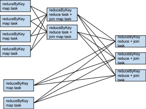
Here is a more complicated transformation graph including a join transformation with multiple dependencies.

The pink boxes show the resulting stage graph used to execute it.

At each stage boundary, data is written to disk by tasks in the parent stages and then fetched over the network by tasks in the child stage. Because they incur heavy disk and network I/O, stage boundaries can be expensive and should be avoided when possible. The number of data partitions in the parent stage may be different than the number of partitions in the child stage. Transformations that may trigger a stage boundary typically accept a numPartitions argument that determines how many partitions to split the data into in the child stage.

Just as the number of reducers is an important parameter in tuning MapReduce jobs, tuning the number of partitions at stage boundaries can often make or break an application’s performance. We’ll delve deeper into how to tune this number in a later section.

Picking the Right Operators

When trying to accomplish something with Spark, a developer can usually choose from many arrangements of actions and transformations that will produce the same results. However, not all these arrangements will result in the same performance: avoiding common pitfalls and picking the right arrangement can make a world of difference in an application’s performance. A few rules and insights will help you orient yourself when these choices come up.

Recent work in SPARK-5097 began stabilizing SchemaRDD, which will open up Spark’s Catalyst optimizer to programmers using Spark’s core APIs, allowing Spark to make some higher-level choices about which operators to use. When SchemaRDD becomes a stable component, users will be shielded from needing to make some of these decisions.

The primary goal when choosing an arrangement of operators is to reduce the number of shuffles and the amount of data shuffled. This is because shuffles are fairly expensive operations; all shuffle data must be written to disk and then transferred over the network. repartition , join, cogroup, and any of the *By or*ByKey transformations can result in shuffles. Not all these operations are equal, however, and a few of the most common performance pitfalls for novice Spark developers arise from picking the wrong one:

Avoid groupByKey when performing an associative reductive operation. For example,rdd.groupByKey().mapValues(_.sum) will produce the same results as rdd.reduceByKey(_ + _). However, the former will transfer the entire dataset across the network, while the latter will compute local sums for each key in each partition and combine those local sums into larger sums after shuffling.

Avoid reduceByKey When the input and output value types are different. For example, consider writing a transformation that finds all the unique strings corresponding to each key. One way would be to use map to transform each element into a Set and then combine the Sets with reduceByKey:

rdd.map(kv => (kv._1, new Set[String]() + kv._2))    .reduceByKey(_ ++ _)

This code results in tons of unnecessary object creation because a new set must be allocated for each record. It’s better to use aggregateByKey, which performs the map-side aggregation more efficiently:

val zero = new collection.mutable.Set[String]()rdd.aggregateByKey(zero)(    (set, v) => set += v,    (set1, set2) => set1 ++= set2)

Avoid the flatMap-join-groupBy pattern. When two datasets are already grouped by key and you want to join them and keep them grouped, you can just use cogroup. That avoids all the overhead associated with unpacking and repacking the groups.

When Shuffles Don’t Happen

It’s also useful to be aware of the cases in which the above transformations will not result in shuffles. Spark knows to avoid a shuffle when a previous transformation has already partitioned the data according to the same partitioner. Consider the following flow:

rdd1 = someRdd.reduceByKey(...)
rdd2 = someOtherRdd.reduceByKey(...)
rdd3 = rdd1.join(rdd2)

Because no partitioner is passed to reduceByKey, the default partitioner will be used, resulting in rdd1 and rdd2 both hash-partitioned. These two reduceByKeys will result in two shuffles. If the RDDs have the same number of partitions, the join will require no additional shuffling. Because the RDDs are partitioned identically, the set of keys in any single partition of rdd1 can only show up in a single partition of rdd2. Therefore, the contents of any single output partition of rdd3 will depend only on the contents of a single partition in rdd1 and single partition in rdd2, and a third shuffle is not required.

For example, if someRdd has four partitions, someOtherRdd has two partitions, and both the reduceByKeys use three partitions, the set of tasks that execute would look like:

What if rdd1 and rdd2 use different partitioners or use the default (hash) partitioner with different numbers partitions?  In that case, only one of the rdds (the one with the fewer number of partitions) will need to be reshuffled for the join.

Same transformations, same inputs, different number of partitions:

One way to avoid shuffles when joining two datasets is to take advantage of broadcast variables. When one of the datasets is small enough to fit in memory in a single executor, it can be loaded into a hash table on the driver and then broadcast to every executor. A map transformation can then reference the hash table to do lookups.

When More Shuffles are Better

There is an occasional exception to the rule of minimizing the number of shuffles. An extra shuffle can be advantageous to performance when it increases parallelism. For example, if your data arrives in a few large unsplittable files, the partitioning dictated by the InputFormat might place large numbers of records in each partition, while not generating enough partitions to take advantage of all the available cores. In this case, invoking repartition with a high number of partitions (which will trigger a shuffle) after loading the data will allow the operations that come after it to leverage more of the cluster’s CPU.

Another instance of this exception can arise when using the reduce or aggregate action to aggregate data into the driver. When aggregating over a high number of partitions, the computation can quickly become bottlenecked on a single thread in the driver merging all the results together. To loosen the load on the driver, one can first use reduceByKey or aggregateByKey to carry out a round of distributed aggregation that divides the dataset into a smaller number of partitions. The values within each partition are merged with each other in parallel, before sending their results to the driver for a final round of aggregation. Take a look at treeReduce and treeAggregate for examples of how to do that. (Note that in 1.2, the most recent version at the time of this writing, these are marked as developer APIs, but SPARK-5430 seeks to add stable versions of them in core.)

This trick is especially useful when the aggregation is already grouped by a key. For example, consider an app that wants to count the occurrences of each word in a corpus and pull the results into the driver as a map.  One approach, which can be accomplished with the aggregate action, is to compute a local map at each partition and then merge the maps at the driver. The alternative approach, which can be accomplished with aggregateByKey, is to perform the count in a fully distributed way, and then simplycollectAsMap the results to the driver.

Secondary Sort

Another important capability to be aware of is the repartitionAndSortWithinPartitions transformation. It’s a transformation that sounds arcane, but seems to come up in all sorts of strange situations. This transformation pushes sorting down into the shuffle machinery, where large amounts of data can be spilled efficiently and sorting can be combined with other operations.

For example, Apache Hive on Spark uses this transformation inside its join implementation. It also acts as a vital building block in the secondary sort pattern, in which you want to both group records by key and then, when iterating over the values that correspond to a key, have them show up in a particular order. This issue comes up in algorithms that need to group events by user and then analyze the events for each user based on the order they occurred in time. Taking advantage of repartitionAndSortWithinPartitionsto do secondary sort currently requires a bit of legwork on the part of the user, but SPARK-3655 will simplify things vastly.

Conclusion

You should now have a good understanding of the basic factors in involved in creating a performance-efficient Spark program! In Part 2, we’ll cover tuning resource requests, parallelism, and data structures.

Sandy Ryza is a Data Scientist at Cloudera, an Apache Spark committer, and an Apache Hadoop PMC member. He is a co-author of the O’Reilly Media book, Advanced Analytics with Spark.