如何用python进行相关性分析_如何利用python进行时间序列分析

题记:毕业一年多天天coding,好久没写paper了。在这动荡的日子里,也希望写点东西让自己静一静。恰好前段时间用python做了一点时间序列方面的东西,有一丁点心得体会想和大家分享下。在此也要特别感谢顾志耐和散沙,让我喜欢上了python。
什么是时间序列
时间序列简单的说就是各时间点上形成的数值序列,时间序列分析就是通过观察历史数据预测未来的值。在这里需要强调一点的是,时间序列分析并不是关于时间的回归,它主要是研究自身的变化规律的(这里不考虑含外生变量的时间序列)。
为什么用python
用两个字总结“情怀”,爱屋及乌,个人比较喜欢python,就用python撸了。能做时间序列的软件很多,SAS、R、SPSS、Eviews甚至matlab等等,实际工作中应用得比较多的应该还是SAS和R,前者推荐王燕写的《应用时间序列分析》,后者推荐“基于R语言的时间序列建模完整教程”这篇博文(翻译版)。python作为科学计算的利器,当然也有相关分析的包:statsmodels中tsa模块,当然这个包和SAS、R是比不了,但是python有另一个神器:pandas!pandas在时间序列上的应用,能简化我们很多的工作。
环境配置
python推荐直接装Anaconda,它集成了许多科学计算包,有一些包自己手动去装还是挺费劲的。statsmodels需要自己去安装,这里我推荐使用0.6的稳定版,0.7及其以上的版本能在github上找到,该版本在安装时会用C编译好,所以修改底层的一些代码将不会起作用。
时间序列分析
1.基本模型
自回归移动平均模型(ARMA(p,q))是时间序列中最为重要的模型之一,它主要由两部分组成: AR代表p阶自回归过程,MA代表q阶移动平均过程,其公式如下:

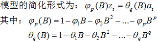
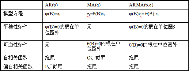
依据模型的形式、特性及自相关和偏自相关函数的特征,总结如下:
在时间序列中,ARIMA模型是在ARMA模型的基础上多了差分的操作。
2.pandas时间序列操作
大熊猫真的很可爱,这里简单介绍一下它在时间序列上的可爱之处。和许多时间序列分析一样,本文同样使用航空乘客数据(AirPassengers.csv)作为样例。
数据读取:
# -*- coding:utf-8 -*-
import numpy as np
import pandas as pdfrom datetime import datetimeimport matplotlib.pylab as plt
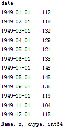
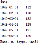
# 读取数据,pd.read_csv默认生成DataFrame对象,需将其转换成Series对象df = pd.read_csv('AirPassengers.csv', encoding='utf-8', index_col='date')df.index = pd.to_datetime(df.index) # 将字符串索引转换成时间索引ts = df['x'] # 生成pd.Series对象# 查看数据格式ts.head()ts.head().index
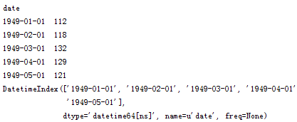
查看某日的值既可以使用字符串作为索引,又可以直接使用时间对象作为索引
ts['1949-01-01']ts[datetime(1949,1,1)]
两者的返回值都是第一个序列值:112
如果要查看某一年的数据,pandas也能非常方便的实现
ts['1949']
切片操作:
ts['1949-1' : '1949-6']
注意时间索引的切片操作起点和尾部都是包含的,这点与数值索引有所不同
pandas还有很多方便的时间序列函数,在后面的实际应用中在进行说明。
3. 平稳性检验
我们知道序列平稳性是进行时间序列分析的前提条件,很多人都会有疑问,为什么要满足平稳性的要求呢?在大数定理和中心定理中要求样本同分布(这里同分布等价于时间序列中的平稳性),而我们的建模过程中有很多都是建立在大数定理和中心极限定理的前提条件下的,如果它不满足,得到的许多结论都是不可靠的。以虚假回归为例,当响应变量和输入变量都平稳时,我们用t统计量检验标准化系数的显著性。而当响应变量和输入变量不平稳时,其标准化系数不在满足t分布,这时再用t检验来进行显著性分析,导致拒绝原假设的概率增加,即容易犯第一类错误,从而得出错误的结论。
平稳时间序列有两种定义:严平稳和宽平稳
严平稳顾名思义,是一种条件非常苛刻的平稳性,它要求序列随着时间的推移,其统计性质保持不变。对于任意的τ,其联合概率密度函数满足:

严平稳的条件只是理论上的存在,现实中用得比较多的是宽平稳的条件。
宽平稳也叫弱平稳或者二阶平稳(均值和方差平稳),它应满足:
常数均值
常数方差
常数自协方差
平稳性检验:观察法和单位根检验法
基于此,我写了一个名为test_stationarity的统计性检验模块,以便将某些统计检验结果更加直观的展现出来。
# -*- coding:utf-8 -*-
from statsmodels.tsa.stattools import adfuller
import pandas as pd
import matplotlib.pyplot as plt
import numpy as np
from statsmodels.graphics.tsaplots import plot_acf, plot_pacf
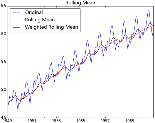
# 移动平均图
def draw_trend(timeSeries, size):
f = plt.figure(facecolor='white')
# 对size个数据进行移动平均
rol_mean = timeSeries.rolling(window=size).mean()
# 对size个数据进行加权移动平均
rol_weighted_mean = pd.ewma(timeSeries, span=size)
timeSeries.plot(color='blue', label='Original')
rolmean.plot(color='red', label='Rolling Mean')
rol_weighted_mean.plot(color='black', label='Weighted Rolling Mean')
plt.legend(loc='best')
plt.title('Rolling Mean')
plt.show()
def draw_ts(timeSeries): f = plt.figure(facecolor='white')
timeSeries.plot(color='blue')
plt.show()
''' Unit Root Test
The null hypothesis of the Augmented Dickey-Fuller is that there is a unit
root, with the alternative that there is no unit root. That is to say the
bigger the p-value the more reason we assert that there is a unit root
'''
def testStationarity(ts):
dftest = adfuller(ts)
# 对上述函数求得的值进行语义描述
dfoutput = pd.Series(dftest[0:4], index=['Test Statistic','p-value','#Lags Used','Number of Observations Used'])
for key,value in dftest[4].items():
dfoutput['Critical Value (%s)'%key] = value
return dfoutput
# 自相关和偏相关图,默认阶数为31阶
def draw_acf_pacf(ts, lags=31):
f = plt.figure(facecolor='white')
ax1 = f.add_subplot(211)
plot_acf(ts, lags=31, ax=ax1)
ax2 = f.add_subplot(212)
plot_pacf(ts, lags=31, ax=ax2)
plt.show()
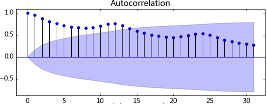
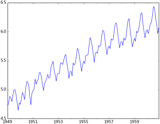
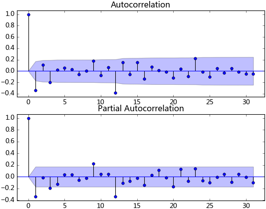
观察法,通俗的说就是通过观察序列的趋势图与相关图是否随着时间的变化呈现出某种规律。所谓的规律就是时间序列经常提到的周期性因素,现实中遇到得比较多的是线性周期成分,这类周期成分可以采用差分或者移动平均来解决,而对于非线性周期成分的处理相对比较复杂,需要采用某些分解的方法。下图为航空数据的线性图,可以明显的看出它具有年周期成分和长期趋势成分。平稳序列的自相关系数会快速衰减,下面的自相关图并不能体现出该特征,所以我们有理由相信该序列是不平稳的。

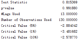
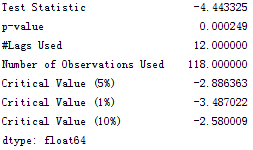
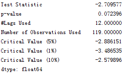
单位根检验:ADF是一种常用的单位根检验方法,他的原假设为序列具有单位根,即非平稳,对于一个平稳的时序数据,就需要在给定的置信水平上显著,拒绝原假设。ADF只是单位根检验的方法之一,如果想采用其他检验方法,可以安装第三方包arch,里面提供了更加全面的单位根检验方法,个人还是比较钟情ADF检验。以下为检验结果,其p值大于0.99,说明并不能拒绝原假设。
3. 平稳性处理
由前面的分析可知,该序列是不平稳的,然而平稳性是时间序列分析的前提条件,故我们需要对不平稳的序列进行处理将其转换成平稳的序列。
a. 对数变换
对数变换主要是为了减小数据的振动幅度,使其线性规律更加明显(我是这么理解的时间序列模型大部分都是线性的,为了尽量降低非线性的因素,需要对其进行预处理,也许我理解的不对)。对数变换相当于增加了一个惩罚机制,数据越大其惩罚越大,数据越小惩罚越小。这里强调一下,变换的序列需要满足大于0,小于0的数据不存在对数变换。
ts_log = np.log(ts)
test_stationarity.draw_ts(ts_log)
b. 平滑法
根据平滑技术的不同,平滑法具体分为移动平均法和指数平均法。
移动平均即利用一定时间间隔内的平均值作为某一期的估计值,而指数平均则是用变权的方法来计算均值
test_stationarity.draw_trend(ts_log, 12)
从上图可以发现窗口为12的移动平均能较好的剔除年周期性因素,而指数平均法是对周期内的数据进行了加权,能在一定程度上减小年周期因素,但并不能完全剔除,如要完全剔除可以进一步进行差分操作。
c. 差分
时间序列最常用来剔除周期性因素的方法当属差分了,它主要是对等周期间隔的数据进行线性求减。前面我们说过,ARIMA模型相对ARMA模型,仅多了差分操作,ARIMA模型几乎是所有时间序列软件都支持的,差分的实现与还原都非常方便。而statsmodel中,对差分的支持不是很好,它不支持高阶和多阶差分,为什么不支持,这里引用作者的说法:
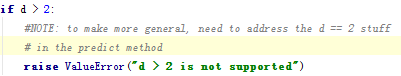
作者大概的意思是说预测方法中并没有解决高于2阶的差分,有没有感觉很牵强,不过没关系,我们有pandas。我们可以先用pandas将序列差分好,然后在对差分好的序列进行ARIMA拟合,只不过这样后面会多了一步人工还原的工作。
diff_12 = ts_log.diff(12)
diff_12.dropna(inplace=True)
diff_12_1 = diff_12.diff(1)
diff_12_1.dropna(inplace=True)
test_stationarity.testStationarity(diff_12_1)
从上面的统计检验结果可以看出,经过12阶差分和1阶差分后,该序列满足平稳性的要求了。
d. 分解
所谓分解就是将时序数据分离成不同的成分。statsmodels使用的X-11分解过程,它主要将时序数据分离成长期趋势、季节趋势和随机成分。与其它统计软件一样,statsmodels也支持两类分解模型,加法模型和乘法模型,这里我只实现加法,乘法只需将model的参数设置为"multiplicative"即可。
from statsmodels.tsa.seasonal import seasonal_decompose
decomposition = seasonal_decompose(ts_log, model="additive")
trend = decomposition.trend
seasonal = decomposition.seasonal
residual = decomposition.resid
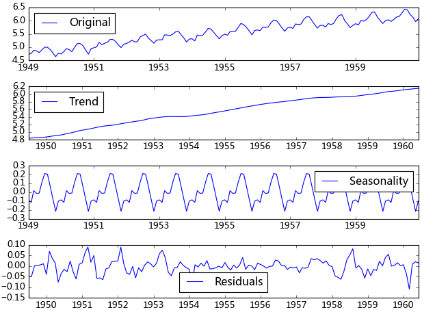
得到不同的分解成分后,就可以使用时间序列模型对各个成分进行拟合,当然也可以选择其他预测方法。我曾经用过小波对时序数据进行过分解,然后分别采用时间序列拟合,效果还不错。由于我对小波的理解不是很好,只能简单的调用接口,如果有谁对小波、傅里叶、卡尔曼理解得比较透,可以将时序数据进行更加准确的分解,由于分解后的时序数据避免了他们在建模时的交叉影响,所以我相信它将有助于预测准确性的提高。
4. 模型识别
在前面的分析可知,该序列具有明显的年周期与长期成分。对于年周期成分我们使用窗口为12的移动平进行处理,对于长期趋势成分我们采用1阶差分来进行处理。
rol_mean = ts_log.rolling(window=12).mean()
rol_mean.dropna(inplace=True)
ts_diff_1 = rol_mean.diff(1)
ts_diff_1.dropna(inplace=True)
test_stationarity.testStationarity(ts_diff_1)
观察其统计量发现该序列在置信水平为95%的区间下并不显著,我们对其进行再次一阶差分。再次差分后的序列其自相关具有快速衰减的特点,t统计量在99%的置信水平下是显著的,这里我不再做详细说明。
ts_diff_2 = ts_diff_1.diff(1)
ts_diff_2.dropna(inplace=True)
数据平稳后,需要对模型定阶,即确定p、q的阶数。观察上图,发现自相关和偏相系数都存在拖尾的特点,并且他们都具有明显的一阶相关性,所以我们设定p=1, q=1。下面就可以使用ARMA模型进行数据拟合了。这里我不使用ARIMA(ts_diff_1, order=(1, 1, 1))进行拟合,是因为含有差分操作时,预测结果还原老出问题,至今还没弄明白。
from statsmodels.tsa.arima_model import ARMA
model = ARMA(ts_diff_2, order=(1, 1))
result_arma = model.fit( disp=-1, method='css')
5. 样本拟合
模型拟合完后,我们就可以对其进行预测了。由于ARMA拟合的是经过相关预处理后的数据,故其预测值需要通过相关逆变换进行还原。
predict_ts = result_arma.predict()
# 一阶差分还原diff_shift_ts = ts_diff_1.shift(1)diff_recover_1 = predict_ts.add(diff_shift_ts)# 再次一阶差分还原
rol_shift_ts = rol_mean.shift(1)
diff_recover = diff_recover_1.add(rol_shift_ts)
# 移动平均还原
rol_sum = ts_log.rolling(window=11).sum()
rol_recover = diff_recover*12 - rol_sum.shift(1)
# 对数还原
log_recover = np.exp(rol_recover)
log_recover.dropna(inplace=True)
我们使用均方根误差(RMSE)来评估模型样本内拟合的好坏。利用该准则进行判别时,需要剔除“非预测”数据的影响。
ts = ts[log_recover.index] # 过滤没有预测的记录plt.figure(facecolor='white')
log_recover.plot(color='blue', label='Predict')
ts.plot(color='red', label='Original')
plt.legend(loc='best')
plt.title('RMSE: %.4f'% np.sqrt(sum((log_recover-ts)**2)/ts.size))
plt.show()
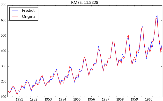
观察上图的拟合效果,均方根误差为11.8828,感觉还过得去。
6.完善ARIMA模型
前面提到statsmodels里面的ARIMA模块不支持高阶差分,我们的做法是将差分分离出来,但是这样会多了一步人工还原的操作。基于上述问题,我将差分过程进行了封装,使序列能按照指定的差分列表依次进行差分,并相应的构造了一个还原的方法,实现差分序列的自动还原。
# 差分操作
def diff_ts(ts, d):
global shift_ts_list
# 动态预测第二日的值时所需要的差分序列
global last_data_shift_list
shift_ts_list = []
last_data_shift_list = []
tmp_ts = ts
for i in d:
last_data_shift_list.append(tmp_ts[-i])
print last_data_shift_list
shift_ts = tmp_ts.shift(i)
shift_ts_list.append(shift_ts)
tmp_ts = tmp_ts - shift_ts
tmp_ts.dropna(inplace=True)
return tmp_ts
# 还原操作
def predict_diff_recover(predict_value, d):
if isinstance(predict_value, float):
tmp_data = predict_value
for i in range(len(d)):
tmp_data = tmp_data + last_data_shift_list[-i-1]
elif isinstance(predict_value, np.ndarray):
tmp_data = predict_value[0]
for i in range(len(d)):
tmp_data = tmp_data + last_data_shift_list[-i-1]
else:
tmp_data = predict_value
for i in range(len(d)):
try:
tmp_data = tmp_data.add(shift_ts_list[-i-1])
except:
raise ValueError('What you input is not pd.Series type!')
tmp_data.dropna(inplace=True)
return tmp_data
现在我们直接使用差分的方法进行数据处理,并以同样的过程进行数据预测与还原。
diffed_ts = diff_ts(ts_log, d=[12, 1])
model = arima_model(diffed_ts)
model.certain_model(1, 1)
predict_ts = model.properModel.predict()
diff_recover_ts = predict_diff_recover(predict_ts, d=[12, 1])
log_recover = np.exp(diff_recover_ts)
是不是发现这里的预测结果和上一篇的使用12阶移动平均的预测结果一模一样。这是因为12阶移动平均加上一阶差分与直接12阶差分是等价的关系,后者是前者数值的12倍,这个应该不难推导。
对于个数不多的时序数据,我们可以通过观察自相关图和偏相关图来进行模型识别,倘若我们要分析的时序数据量较多,例如要预测每只股票的走势,我们就不可能逐个去调参了。这时我们可以依据BIC准则识别模型的p, q值,通常认为BIC值越小的模型相对更优。这里我简单介绍一下BIC准则,它综合考虑了残差大小和自变量的个数,残差越小BIC值越小,自变量个数越多BIC值越大。个人觉得BIC准则就是对模型过拟合设定了一个标准(过拟合这东西应该以辩证的眼光看待)。
def proper_model(data_ts, maxLag):
init_bic = sys.maxint
init_p = 0
init_q = 0
init_properModel = None
for p in np.arange(maxLag):
for q in np.arange(maxLag):
model = ARMA(data_ts, order=(p, q))
try:
results_ARMA = model.fit(disp=-1, method='css')
except:
continue
bic = results_ARMA.bic
if bic < init_bic:
init_p = p
init_q = q
init_properModel = results_ARMA
init_bic = bic
return init_bic, init_p, init_q, init_properModel
相对最优参数识别结果:BIC: -1090.44209358 p: 0 q: 1 ,RMSE:11.8817198331。我们发现模型自动识别的参数要比我手动选取的参数更优。
7.滚动预测
所谓滚动预测是指通过添加最新的数据预测第二天的值。对于一个稳定的预测模型,不需要每天都去拟合,我们可以给他设定一个阀值,例如每周拟合一次,该期间只需通过添加最新的数据实现滚动预测即可。基于此我编写了一个名为arima_model的类,主要包含模型自动识别方法,滚动预测的功能,详细代码可以查看附录。数据的动态添加:
from dateutil.relativedelta import relativedeltadef _add_new_data(ts, dat, type='day'):
if type == 'day':
new_index = ts.index[-1] + relativedelta(days=1)
elif type == 'month':
new_index = ts.index[-1] + relativedelta(months=1)
ts[new_index] = dat
def add_today_data(model, ts, data, d, type='day'):
_add_new_data(ts, data, type) # 为原始序列添加数据
# 为滞后序列添加新值
d_ts = diff_ts(ts, d)
model.add_today_data(d_ts[-1], type)
def forecast_next_day_data(model, type='day'):
if model == None:
raise ValueError('No model fit before')
fc = model.forecast_next_day_value(type)
return predict_diff_recover(fc, [12, 1])
现在我们就可以使用滚动预测的方法向外预测了,取1957年之前的数据作为训练数据,其后的数据作为测试,并设定模型每第七天就会重新拟合一次。这里的diffed_ts对象会随着add_today_data方法自动添加数据,这是由于它与add_today_data方法中的d_ts指向的同一对象,该对象会动态的添加数据。
ts_train = ts_log[:'1956-12']
ts_test = ts_log['1957-1':]
diffed_ts = diff_ts(ts_train, [12, 1])
forecast_list = []
for i, dta in enumerate(ts_test):
if i%7 == 0:
model = arima_model(diffed_ts)
model.certain_model(1, 1)
forecast_data = forecast_next_day_data(model, type='month')
forecast_list.append(forecast_data)
add_today_data(model, ts_train, dta, [12, 1], type='month')
predict_ts = pd.Series(data=forecast_list, index=ts['1957-1':].index)log_recover = np.exp(predict_ts)original_ts = ts['1957-1':]
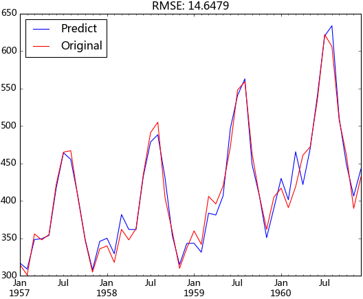
动态预测的均方根误差为:14.6479,与前面样本内拟合的均方根误差相差不大,说明模型并没有过拟合,并且整体预测效果都较好。
8. 模型序列化
在进行动态预测时,我们不希望将整个模型一直在内存中运行,而是希望有新的数据到来时才启动该模型。这时我们就应该把整个模型从内存导出到硬盘中,而序列化正好能满足该要求。序列化最常用的就是使用json模块了,但是它是时间对象支持得不是很好,有人对json模块进行了拓展以使得支持时间对象,这里我们不采用该方法,我们使用pickle模块,它和json的接口基本相同,有兴趣的可以去查看一下。我在实际应用中是采用的面向对象的编程,它的序列化主要是将类的属性序列化即可,而在面向过程的编程中,模型序列化需要将需要序列化的对象公有化,这样会使得对前面函数的参数改动较大,我不在详细阐述该过程。
总结
与其它统计语言相比,python在统计分析这块还显得不那么“专业”。随着numpy、pandas、scipy、sklearn、gensim、statsmodels等包的推动,我相信也祝愿python在数据分析这块越来越好。与SAS和R相比,python的时间序列模块还不是很成熟,我这里仅起到抛砖引玉的作用,希望各位能人志士能贡献自己的力量,使其更加完善。实际应用中我全是面向过程来编写的,为了阐述方便,我用面向过程重新罗列了一遍,实在感觉很不方便。原本打算分三篇来写的,还有一部分实际应用的部分,不打算再写了,还请大家原谅。实际应用主要是具体问题具体分析,这当中第一步就是要查询问题,这步花的时间往往会比较多,然后再是解决问题。以我前面项目遇到的问题为例,当时遇到了以下几个典型的问题:1.周期长度不恒定的周期成分,例如每月的1号具有周期性,但每月1号与1号之间的时间间隔是不相等的;2.含有缺失值以及含有记录为0的情况无法进行对数变换;3.节假日的影响等等。
附录
# -*-coding:utf-8-*-
import pandas as pd
import numpy as np
from statsmodels.tsa.arima_model import ARMA
import sys
from dateutil.relativedelta import relativedelta
from copy import deepcopy
import matplotlib.pyplot as plt
class arima_model:
def __init__(self, ts, maxLag=9):
self.data_ts = ts
self.resid_ts = None
self.predict_ts = None
self.maxLag = maxLag
self.p = maxLag
self.q = maxLag
self.properModel = None
self.bic = sys.maxint
# 计算最优ARIMA模型,将相关结果赋给相应属性
def get_proper_model(self):
self._proper_model()
self.predict_ts = deepcopy(self.properModel.predict())
self.resid_ts = deepcopy(self.properModel.resid)
# 对于给定范围内的p,q计算拟合得最好的arima模型,这里是对差分好的数据进行拟合,故差分恒为0
def _proper_model(self):
for p in np.arange(self.maxLag):
for q in np.arange(self.maxLag):
# print p,q,self.bic
model = ARMA(self.data_ts, order=(p, q))
try:
results_ARMA = model.fit(disp=-1, method='css')
except:
continue
bic = results_ARMA.bic
# print 'bic:',bic,'self.bic:',self.bic
if bic < self.bic:
self.p = p
self.q = q
self.properModel = results_ARMA
self.bic = bic
self.resid_ts = deepcopy(self.properModel.resid)
self.predict_ts = self.properModel.predict()
# 参数确定模型
def certain_model(self, p, q):
model = ARMA(self.data_ts, order=(p, q))
try:
self.properModel = model.fit( disp=-1, method='css')
self.p = p
self.q = q
self.bic = self.properModel.bic
self.predict_ts = self.properModel.predict()
self.resid_ts = deepcopy(self.properModel.resid)
except:
print 'You can not fit the model with this parameter p,q, ' \
'please use the get_proper_model method to get the best model'
# 预测第二日的值
def forecast_next_day_value(self, type='day'):
# 我修改了statsmodels包中arima_model的源代码,添加了constant属性,需要先运行forecast方法,为constant赋值
self.properModel.forecast()
if self.data_ts.index[-1] != self.resid_ts.index[-1]:
raise ValueError('''The index is different in data_ts and resid_ts, please add new data to data_ts.
If you just want to forecast the next day data without add the real next day data to data_ts,
please run the predict method which arima_model included itself''')
if not self.properModel:
raise ValueError('The arima model have not computed, please run the proper_model method before')
para = self.properModel.params
# print self.properModel.params
if self.p == 0: # It will get all the value series with setting self.data_ts[-self.p:] when p is zero
ma_value = self.resid_ts[-self.q:]
values = ma_value.reindex(index=ma_value.index[::-1])
elif self.q == 0:
ar_value = self.data_ts[-self.p:]
values = ar_value.reindex(index=ar_value.index[::-1])
else:
ar_value = self.data_ts[-self.p:]
ar_value = ar_value.reindex(index=ar_value.index[::-1])
ma_value = self.resid_ts[-self.q:]
ma_value = ma_value.reindex(index=ma_value.index[::-1])
values = ar_value.append(ma_value)
predict_value = np.dot(para[1:], values) + self.properModel.constant[0]
self._add_new_data(self.predict_ts, predict_value, type)
return predict_value
# 动态添加数据函数,针对索引是月份和日分别进行处理
def _add_new_data(self, ts, dat, type='day'):
if type == 'day':
new_index = ts.index[-1] + relativedelta(days=1)
elif type == 'month':
new_index = ts.index[-1] + relativedelta(months=1)
ts[new_index] = dat
def add_today_data(self, dat, type='day'):
self._add_new_data(self.data_ts, dat, type)
if self.data_ts.index[-1] != self.predict_ts.index[-1]:
raise ValueError('You must use the forecast_next_day_value method forecast the value of today before')
self._add_new_data(self.resid_ts, self.data_ts[-1] - self.predict_ts[-1], type)
if __name__ == '__main__':
df = pd.read_csv('AirPassengers.csv', encoding='utf-8', index_col='date')
df.index = pd.to_datetime(df.index)
ts = df['x']
# 数据预处理
ts_log = np.log(ts)
rol_mean = ts_log.rolling(window=12).mean()
rol_mean.dropna(inplace=True)
ts_diff_1 = rol_mean.diff(1)
ts_diff_1.dropna(inplace=True)
ts_diff_2 = ts_diff_1.diff(1)
ts_diff_2.dropna(inplace=True)
# 模型拟合
model = arima_model(ts_diff_2)
# 这里使用模型参数自动识别
model.get_proper_model()
print 'bic:', model.bic, 'p:', model.p, 'q:', model.q
print model.properModel.forecast()[0]
print model.forecast_next_day_value(type='month')
# 预测结果还原
predict_ts = model.properModel.predict()
diff_shift_ts = ts_diff_1.shift(1)
diff_recover_1 = predict_ts.add(diff_shift_ts)
rol_shift_ts = rol_mean.shift(1)
diff_recover = diff_recover_1.add(rol_shift_ts)
rol_sum = ts_log.rolling(window=11).sum()
rol_recover = diff_recover*12 - rol_sum.shift(1)
log_recover = np.exp(rol_recover)
log_recover.dropna(inplace=True)
# 预测结果作图
ts = ts[log_recover.index]
plt.figure(facecolor='white')
log_recover.plot(color='blue', label='Predict')
ts.plot(color='red', label='Original')
plt.legend(loc='best')
plt.title('RMSE: %.4f'% np.sqrt(sum((log_recover-ts)**2)/ts.size))
plt.show()
修改的arima_model代码
# Note: The information criteria add 1 to the number of parameters
# whenever the model has an AR or MA term since, in principle,
# the variance could be treated as a free parameter and restricted
# This code does not allow this, but it adds consistency with other
# packages such as gretl and X12-ARIMA
from __future__ import absolute_import
from statsmodels.compat.python import string_types, range
# for 2to3 with extensions
from datetime import datetime
import numpy as np
from scipy import optimize
from scipy.stats import t, norm
from scipy.signal import lfilter
from numpy import dot, log, zeros, pi
from numpy.linalg import inv
from statsmodels.tools.decorators import (cache_readonly,
resettable_cache)
import statsmodels.tsa.base.tsa_model as tsbase
import statsmodels.base.wrapper as wrap
from statsmodels.regression.linear_model import yule_walker, GLS
from statsmodels.tsa.tsatools import (lagmat, add_trend,
_ar_transparams, _ar_invtransparams,
_ma_transparams, _ma_invtransparams,
unintegrate, unintegrate_levels)
from statsmodels.tsa.vector_ar import util
from statsmodels.tsa.ar_model import AR
from statsmodels.tsa.arima_process import arma2ma
from statsmodels.tools.numdiff import approx_hess_cs, approx_fprime_cs
from statsmodels.tsa.base.datetools import _index_date
from statsmodels.tsa.kalmanf import KalmanFilter
_armax_notes = """
Notes
-----
If exogenous variables are given, then the model that is fit is
.. math::
\\phi(L)(y_t - X_t\\beta) = \\theta(L)\epsilon_t
where :math:`\\phi` and :math:`\\theta` are polynomials in the lag
operator, :math:`L`. This is the regression model with ARMA errors,
or ARMAX model. This specification is used, whether or not the model
is fit using conditional sum of square or maximum-likelihood, using
the `method` argument in
:meth:`statsmodels.tsa.arima_model.%(Model)s.fit`. Therefore, for
now, `css` and `mle` refer to estimation methods only. This may
change for the case of the `css` model in future versions.
"""
_arma_params = """\
endog : array-like
The endogenous variable.
order : iterable
The (p,q) order of the model for the number of AR parameters,
differences, and MA parameters to use.
exog : array-like, optional
An optional arry of exogenous variables. This should *not* include a
constant or trend. You can specify this in the `fit` method."""
_arma_model = "Autoregressive Moving Average ARMA(p,q) Model"
_arima_model = "Autoregressive Integrated Moving Average ARIMA(p,d,q) Model"
_arima_params = """\
endog : array-like
The endogenous variable.
order : iterable
The (p,d,q) order of the model for the number of AR parameters,
differences, and MA parameters to use.
exog : array-like, optional
An optional arry of exogenous variables. This should *not* include a
constant or trend. You can specify this in the `fit` method."""
_predict_notes = """
Notes
-----
Use the results predict method instead.
"""
_results_notes = """
Notes
-----
It is recommended to use dates with the time-series models, as the
below will probably make clear. However, if ARIMA is used without
dates and/or `start` and `end` are given as indices, then these
indices are in terms of the *original*, undifferenced series. Ie.,
given some undifferenced observations::
1970Q1, 1
1970Q2, 1.5
1970Q3, 1.25
1970Q4, 2.25
1971Q1, 1.2
1971Q2, 4.1
1970Q1 is observation 0 in the original series. However, if we fit an
ARIMA(p,1,q) model then we lose this first observation through
differencing. Therefore, the first observation we can forecast (if
using exact MLE) is index 1. In the differenced series this is index
0, but we refer to it as 1 from the original series.
"""
_predict = """
%(Model)s model in-sample and out-of-sample prediction
Parameters
----------
%(params)s
start : int, str, or datetime
Zero-indexed observation number at which to start forecasting, ie.,
the first forecast is start. Can also be a date string to
parse or a datetime type.
end : int, str, or datetime
Zero-indexed observation number at which to end forecasting, ie.,
the first forecast is start. Can also be a date string to
parse or a datetime type. However, if the dates index does not
have a fixed frequency, end must be an integer index if you
want out of sample prediction.
exog : array-like, optional
If the model is an ARMAX and out-of-sample forecasting is
requested, exog must be given. Note that you'll need to pass
`k_ar` additional lags for any exogenous variables. E.g., if you
fit an ARMAX(2, q) model and want to predict 5 steps, you need 7
observations to do this.
dynamic : bool, optional
The `dynamic` keyword affects in-sample prediction. If dynamic
is False, then the in-sample lagged values are used for
prediction. If `dynamic` is True, then in-sample forecasts are
used in place of lagged dependent variables. The first forecasted
value is `start`.
%(extra_params)s
Returns
-------
%(returns)s
%(extra_section)s
"""
_predict_returns = """predict : array
The predicted values.
"""
_arma_predict = _predict % {"Model" : "ARMA",
"params" : """
params : array-like
The fitted parameters of the model.""",
"extra_params" : "",
"returns" : _predict_returns,
"extra_section" : _predict_notes}
_arma_results_predict = _predict % {"Model" : "ARMA", "params" : "",
"extra_params" : "",
"returns" : _predict_returns,
"extra_section" : _results_notes}
_arima_predict = _predict % {"Model" : "ARIMA",
"params" : """params : array-like
The fitted parameters of the model.""",
"extra_params" : """typ : str {'linear', 'levels'}
- 'linear' : Linear prediction in terms of the differenced
endogenous variables.
- 'levels' : Predict the levels of the original endogenous
variables.\n""", "returns" : _predict_returns,
"extra_section" : _predict_notes}
_arima_results_predict = _predict % {"Model" : "ARIMA",
"params" : "",
"extra_params" :
"""typ : str {'linear', 'levels'}
- 'linear' : Linear prediction in terms of the differenced
endogenous variables.
- 'levels' : Predict the levels of the original endogenous
variables.\n""",
"returns" : _predict_returns,
"extra_section" : _results_notes}
_arima_plot_predict_example = """ Examples
--------
>>> import statsmodels.api as sm
>>> import matplotlib.pyplot as plt
>>> import pandas as pd
>>>
>>> dta = sm.datasets.sunspots.load_pandas().data[['SUNACTIVITY']]
>>> dta.index = pd.DatetimeIndex(start='1700', end='2009', freq='A')
>>> res = sm.tsa.ARMA(dta, (3, 0)).fit()
>>> fig, ax = plt.subplots()
>>> ax = dta.ix['1950':].plot(ax=ax)
>>> fig = res.plot_predict('1990', '2012', dynamic=True, ax=ax,
... plot_insample=False)
>>> plt.show()
.. plot:: plots/arma_predict_plot.py
"""
_plot_predict = ("""
Plot forecasts
""" + '\n'.join(_predict.split('\n')[2:])) % {
"params" : "",
"extra_params" : """alpha : float, optional
The confidence intervals for the forecasts are (1 - alpha)%
plot_insample : bool, optional
Whether to plot the in-sample series. Default is True.
ax : matplotlib.Axes, optional
Existing axes to plot with.""",
"returns" : """fig : matplotlib.Figure
The plotted Figure instance""",
"extra_section" : ('\n' + _arima_plot_predict_example +
'\n' + _results_notes)
}
_arima_plot_predict = ("""
Plot forecasts
""" + '\n'.join(_predict.split('\n')[2:])) % {
"params" : "",
"extra_params" : """alpha : float, optional
The confidence intervals for the forecasts are (1 - alpha)%
plot_insample : bool, optional
Whether to plot the in-sample series. Default is True.
ax : matplotlib.Axes, optional
Existing axes to plot with.""",
"returns" : """fig : matplotlib.Figure
The plotted Figure instance""",
"extra_section" : ('\n' + _arima_plot_predict_example +
'\n' +
'\n'.join(_results_notes.split('\n')[:3]) +
("""
This is hard-coded to only allow plotting of the forecasts in levels.
""") +
'\n'.join(_results_notes.split('\n')[3:]))
}
def cumsum_n(x, n):
if n:
n -= 1
x = np.cumsum(x)
return cumsum_n(x, n)
else:
return x
def _check_arima_start(start, k_ar, k_diff, method, dynamic):
if start < 0:
raise ValueError("The start index %d of the original series "
"has been differenced away" % start)
elif (dynamic or 'mle' not in method) and start < k_ar:
raise ValueError("Start must be >= k_ar for conditional MLE "
"or dynamic forecast. Got %d" % start)
def _get_predict_out_of_sample(endog, p, q, k_trend, k_exog, start, errors,
trendparam, exparams, arparams, maparams, steps,
method, exog=None):
"""
Returns endog, resid, mu of appropriate length for out of sample
prediction.
"""
if q:
resid = np.zeros(q)
if start and 'mle' in method or (start == p and not start == 0):
resid[:q] = errors[start-q:start]
elif start:
resid[:q] = errors[start-q-p:start-p]
else:
resid[:q] = errors[-q:]
else:
resid = None
y = endog
if k_trend == 1:
# use expectation not constant
if k_exog > 0:
#TODO: technically should only hold for MLE not
# conditional model. See #274.
# ensure 2-d for conformability
if np.ndim(exog) == 1 and k_exog == 1:
# have a 1d series of observations -> 2d
exog = exog[:, None]
elif np.ndim(exog) == 1:
# should have a 1d row of exog -> 2d
if len(exog) != k_exog:
raise ValueError("1d exog given and len(exog) != k_exog")
exog = exog[None, :]
X = lagmat(np.dot(exog, exparams), p, original='in', trim='both')
mu = trendparam * (1 - arparams.sum())
# arparams were reversed in unpack for ease later
mu = mu + (np.r_[1, -arparams[::-1]] * X).sum(1)[:, None]
else:
mu = trendparam * (1 - arparams.sum())
mu = np.array([mu]*steps)
elif k_exog > 0:
X = np.dot(exog, exparams)
#NOTE: you shouldn't have to give in-sample exog!
X = lagmat(X, p, original='in', trim='both')
mu = (np.r_[1, -arparams[::-1]] * X).sum(1)[:, None]
else:
mu = np.zeros(steps)
endog = np.zeros(p + steps - 1)
if p and start:
endog[:p] = y[start-p:start]
elif p:
endog[:p] = y[-p:]
return endog, resid, mu
def _arma_predict_out_of_sample(params, steps, errors, p, q, k_trend, k_exog,
endog, exog=None, start=0, method='mle'):
(trendparam, exparams,
arparams, maparams) = _unpack_params(params, (p, q), k_trend,
k_exog, reverse=True)
# print 'params:',params
# print 'arparams:',arparams,'maparams:',maparams
endog, resid, mu = _get_predict_out_of_sample(endog, p, q, k_trend, k_exog,
start, errors, trendparam,
exparams, arparams,
maparams, steps, method,
exog)
# print 'mu[-1]:',mu[-1], 'mu[0]:',mu[0]
forecast = np.zeros(steps)
if steps == 1:
if q:
return mu[0] + np.dot(arparams, endog[:p]) + np.dot(maparams,
resid[:q]), mu[0]
else:
return mu[0] + np.dot(arparams, endog[:p]), mu[0]
if q:
i = 0 # if q == 1
else:
i = -1
for i in range(min(q, steps - 1)):
fcast = (mu[i] + np.dot(arparams, endog[i:i + p]) +
np.dot(maparams[:q - i], resid[i:i + q]))
forecast[i] = fcast
endog[i+p] = fcast
for i in range(i + 1, steps - 1):
fcast = mu[i] + np.dot(arparams, endog[i:i+p])
forecast[i] = fcast
endog[i+p] = fcast
#need to do one more without updating endog
forecast[-1] = mu[-1] + np.dot(arparams, endog[steps - 1:])
return forecast, mu[-1] #Modified by me, the former is return forecast
def _arma_predict_in_sample(start, end, endog, resid, k_ar, method):
"""
Pre- and in-sample fitting for ARMA.
"""
if 'mle' in method:
fittedvalues = endog - resid # get them all then trim
else:
fittedvalues = endog[k_ar:] - resid
fv_start = start
if 'mle' not in method:
fv_start -= k_ar # start is in terms of endog index
fv_end = min(len(fittedvalues), end + 1)
return fittedvalues[fv_start:fv_end]
def _validate(start, k_ar, k_diff, dates, method):
if isinstance(start, (string_types, datetime)):
start = _index_date(start, dates)
start -= k_diff
if 'mle' not in method and start < k_ar - k_diff:
raise ValueError("Start must be >= k_ar for conditional "
"MLE or dynamic forecast. Got %s" % start)
return start
def _unpack_params(params, order, k_trend, k_exog, reverse=False):
p, q = order
k = k_trend + k_exog
maparams = params[k+p:]
arparams = params[k:k+p]
trend = params[:k_trend]
exparams = params[k_trend:k]
if reverse:
return trend, exparams, arparams[::-1], maparams[::-1]
return trend, exparams, arparams, maparams
def _unpack_order(order):
k_ar, k_ma, k = order
k_lags = max(k_ar, k_ma+1)
return k_ar, k_ma, order, k_lags
def _make_arma_names(data, k_trend, order, exog_names):
k_ar, k_ma = order
exog_names = exog_names or []
ar_lag_names = util.make_lag_names([data.ynames], k_ar, 0)
ar_lag_names = [''.join(('ar.', i)) for i in ar_lag_names]
ma_lag_names = util.make_lag_names([data.ynames], k_ma, 0)
ma_lag_names = [''.join(('ma.', i)) for i in ma_lag_names]
trend_name = util.make_lag_names('', 0, k_trend)
exog_names = trend_name + exog_names + ar_lag_names + ma_lag_names
return exog_names
def _make_arma_exog(endog, exog, trend):
k_trend = 1 # overwritten if no constant
if exog is None and trend == 'c': # constant only
exog = np.ones((len(endog), 1))
elif exog is not None and trend == 'c': # constant plus exogenous
exog = add_trend(exog, trend='c', prepend=True)
elif exog is not None and trend == 'nc':
# make sure it's not holding constant from last run
if exog.var() == 0:
exog = None
k_trend = 0
if trend == 'nc':
k_trend = 0
return k_trend, exog
def _check_estimable(nobs, n_params):
if nobs <= n_params:
raise ValueError("Insufficient degrees of freedom to estimate")
class ARMA(tsbase.TimeSeriesModel):
__doc__ = tsbase._tsa_doc % {"model" : _arma_model,
"params" : _arma_params, "extra_params" : "",
"extra_sections" : _armax_notes %
{"Model" : "ARMA"}}
def __init__(self, endog, order, exog=None, dates=None, freq=None,
missing='none'):
super(ARMA, self).__init__(endog, exog, dates, freq, missing=missing)
exog = self.data.exog # get it after it's gone through processing
_check_estimable(len(self.endog), sum(order))
self.k_ar = k_ar = order[0]
self.k_ma = k_ma = order[1]
self.k_lags = max(k_ar, k_ma+1)
self.constant = 0 #Added by me
if exog is not None:
if exog.ndim == 1:
exog = exog[:, None]
k_exog = exog.shape[1] # number of exog. variables excl. const
else:
k_exog = 0
self.k_exog = k_exog
def _fit_start_params_hr(self, order):
"""
Get starting parameters for fit.
Parameters
----------
order : iterable
(p,q,k) - AR lags, MA lags, and number of exogenous variables
including the constant.
Returns
-------
start_params : array
A first guess at the starting parameters.
Notes
-----
If necessary, fits an AR process with the laglength selected according
to best BIC. Obtain the residuals. Then fit an ARMA(p,q) model via
OLS using these residuals for a first approximation. Uses a separate
OLS regression to find the coefficients of exogenous variables.
References
----------
Hannan, E.J. and Rissanen, J. 1982. "Recursive estimation of mixed
autoregressive-moving average order." `Biometrika`. 69.1.
"""
p, q, k = order
start_params = zeros((p+q+k))
endog = self.endog.copy() # copy because overwritten
exog = self.exog
if k != 0:
ols_params = GLS(endog, exog).fit().params
start_params[:k] = ols_params
endog -= np.dot(exog, ols_params).squeeze()
if q != 0:
if p != 0:
# make sure we don't run into small data problems in AR fit
nobs = len(endog)
maxlag = int(round(12*(nobs/100.)**(1/4.)))
if maxlag >= nobs:
maxlag = nobs - 1
armod = AR(endog).fit(ic='bic', trend='nc', maxlag=maxlag)
arcoefs_tmp = armod.params
p_tmp = armod.k_ar
# it's possible in small samples that optimal lag-order
# doesn't leave enough obs. No consistent way to fix.
if p_tmp + q >= len(endog):
raise ValueError("Proper starting parameters cannot"
" be found for this order with this "
"number of observations. Use the "
"start_params argument.")
resid = endog[p_tmp:] - np.dot(lagmat(endog, p_tmp,
trim='both'),
arcoefs_tmp)
if p < p_tmp + q:
endog_start = p_tmp + q - p
resid_start = 0
else:
endog_start = 0
resid_start = p - p_tmp - q
lag_endog = lagmat(endog, p, 'both')[endog_start:]
lag_resid = lagmat(resid, q, 'both')[resid_start:]
# stack ar lags and resids
X = np.column_stack((lag_endog, lag_resid))
coefs = GLS(endog[max(p_tmp + q, p):], X).fit().params
start_params[k:k+p+q] = coefs
else:
start_params[k+p:k+p+q] = yule_walker(endog, order=q)[0]
if q == 0 and p != 0:
arcoefs = yule_walker(endog, order=p)[0]
start_params[k:k+p] = arcoefs
# check AR coefficients
if p and not np.all(np.abs(np.roots(np.r_[1, -start_params[k:k + p]]
)) < 1):
raise ValueError("The computed initial AR coefficients are not "
"stationary\nYou should induce stationarity, "
"choose a different model order, or you can\n"
"pass your own start_params.")
# check MA coefficients
elif q and not np.all(np.abs(np.roots(np.r_[1, start_params[k + p:]]
)) < 1):
return np.zeros(len(start_params)) #modified by me
raise ValueError("The computed initial MA coefficients are not "
"invertible\nYou should induce invertibility, "
"choose a different model order, or you can\n"
"pass your own start_params.")
# check MA coefficients
# print start_params
return start_params
def _fit_start_params(self, order, method):
if method != 'css-mle': # use Hannan-Rissanen to get start params
start_params = self._fit_start_params_hr(order)
else: # use CSS to get start params
func = lambda params: -self.loglike_css(params)
#start_params = [.1]*(k_ar+k_ma+k_exog) # different one for k?
start_params = self._fit_start_params_hr(order)
if self.transparams:
start_params = self._invtransparams(start_params)
bounds = [(None,)*2]*sum(order)
mlefit = optimize.fmin_l_bfgs_b(func, start_params,
approx_grad=True, m=12,
pgtol=1e-7, factr=1e3,
bounds=bounds, iprint=-1)
start_params = self._transparams(mlefit[0])
return start_params
def score(self, params):
"""
Compute the score function at params.
Notes
-----
This is a numerical approximation.
"""
return approx_fprime_cs(params, self.loglike, args=(False,))
def hessian(self, params):
"""
Compute the Hessian at params,
Notes
-----
This is a numerical approximation.
"""
return approx_hess_cs(params, self.loglike, args=(False,))
def _transparams(self, params):
"""
Transforms params to induce stationarity/invertability.
Reference
---------
Jones(1980)
"""
k_ar, k_ma = self.k_ar, self.k_ma
k = self.k_exog + self.k_trend
newparams = np.zeros_like(params)
# just copy exogenous parameters
if k != 0:
newparams[:k] = params[:k]
# AR Coeffs
if k_ar != 0:
newparams[k:k+k_ar] = _ar_transparams(params[k:k+k_ar].copy())
# MA Coeffs
if k_ma != 0:
newparams[k+k_ar:] = _ma_transparams(params[k+k_ar:].copy())
return newparams
def _invtransparams(self, start_params):
"""
Inverse of the Jones reparameterization
"""
k_ar, k_ma = self.k_ar, self.k_ma
k = self.k_exog + self.k_trend
newparams = start_params.copy()
arcoefs = newparams[k:k+k_ar]
macoefs = newparams[k+k_ar:]
# AR coeffs
if k_ar != 0:
newparams[k:k+k_ar] = _ar_invtransparams(arcoefs)
# MA coeffs
if k_ma != 0:
newparams[k+k_ar:k+k_ar+k_ma] = _ma_invtransparams(macoefs)
return newparams
def _get_predict_start(self, start, dynamic):
# do some defaults
method = getattr(self, 'method', 'mle')
k_ar = getattr(self, 'k_ar', 0)
k_diff = getattr(self, 'k_diff', 0)
if start is None:
if 'mle' in method and not dynamic:
start = 0
else:
start = k_ar
self._set_predict_start_date(start) # else it's done in super
elif isinstance(start, int):
start = super(ARMA, self)._get_predict_start(start)
else: # should be on a date
#elif 'mle' not in method or dynamic: # should be on a date
start = _validate(start, k_ar, k_diff, self.data.dates,
method)
start = super(ARMA, self)._get_predict_start(start)
_check_arima_start(start, k_ar, k_diff, method, dynamic)
return start
def _get_predict_end(self, end, dynamic=False):
# pass through so predict works for ARIMA and ARMA
return super(ARMA, self)._get_predict_end(end)
def geterrors(self, params):
"""
Get the errors of the ARMA process.
Parameters
----------
params : array-like
The fitted ARMA parameters
order : array-like
3 item iterable, with the number of AR, MA, and exogenous
parameters, including the trend
"""
#start = self._get_predict_start(start) # will be an index of a date
#end, out_of_sample = self._get_predict_end(end)
params = np.asarray(params)
k_ar, k_ma = self.k_ar, self.k_ma
k = self.k_exog + self.k_trend
method = getattr(self, 'method', 'mle')
if 'mle' in method: # use KalmanFilter to get errors
(y, k, nobs, k_ar, k_ma, k_lags, newparams, Z_mat, m, R_mat,
T_mat, paramsdtype) = KalmanFilter._init_kalman_state(params,
self)
errors = KalmanFilter.geterrors(y, k, k_ar, k_ma, k_lags, nobs,
Z_mat, m, R_mat, T_mat,
paramsdtype)
if isinstance(errors, tuple):
errors = errors[0] # non-cython version returns a tuple
else: # use scipy.signal.lfilter
y = self.endog.copy()
k = self.k_exog + self.k_trend
if k > 0:
y -= dot(self.exog, params[:k])
k_ar = self.k_ar
k_ma = self.k_ma
(trendparams, exparams,
arparams, maparams) = _unpack_params(params, (k_ar, k_ma),
self.k_trend, self.k_exog,
reverse=False)
b, a = np.r_[1, -arparams], np.r_[1, maparams]
zi = zeros((max(k_ar, k_ma)))
for i in range(k_ar):
zi[i] = sum(-b[:i+1][::-1]*y[:i+1])
e = lfilter(b, a, y, zi=zi)
errors = e[0][k_ar:]
return errors.squeeze()
def predict(self, params, start=None, end=None, exog=None, dynamic=False):
method = getattr(self, 'method', 'mle') # don't assume fit
#params = np.asarray(params)
# will return an index of a date
start = self._get_predict_start(start, dynamic)
end, out_of_sample = self._get_predict_end(end, dynamic)
if out_of_sample and (exog is None and self.k_exog > 0):
raise ValueError("You must provide exog for ARMAX")
endog = self.endog
resid = self.geterrors(params)
k_ar = self.k_ar
if out_of_sample != 0 and self.k_exog > 0:
if self.k_exog == 1 and exog.ndim == 1:
exog = exog[:, None]
# we need the last k_ar exog for the lag-polynomial
if self.k_exog > 0 and k_ar > 0:
# need the last k_ar exog for the lag-polynomial
exog = np.vstack((self.exog[-k_ar:, self.k_trend:], exog))
if dynamic:
#TODO: now that predict does dynamic in-sample it should
# also return error estimates and confidence intervals
# but how? len(endog) is not tot_obs
out_of_sample += end - start + 1
pr, ct = _arma_predict_out_of_sample(params, out_of_sample, resid,
k_ar, self.k_ma, self.k_trend,
self.k_exog, endog, exog,
start, method)
self.constant = ct
return pr
predictedvalues = _arma_predict_in_sample(start, end, endog, resid,
k_ar, method)
if out_of_sample:
forecastvalues, ct = _arma_predict_out_of_sample(params, out_of_sample,
resid, k_ar,
self.k_ma,
self.k_trend,
self.k_exog, endog,
exog, method=method)
self.constant = ct
predictedvalues = np.r_[predictedvalues, forecastvalues]
return predictedvalues
predict.__doc__ = _arma_predict
def loglike(self, params, set_sigma2=True):
"""
Compute the log-likelihood for ARMA(p,q) model
Notes
-----
Likelihood used depends on the method set in fit
"""
method = self.method
if method in ['mle', 'css-mle']:
return self.loglike_kalman(params, set_sigma2)
elif method == 'css':
return self.loglike_css(params, set_sigma2)
else:
raise ValueError("Method %s not understood" % method)
def loglike_kalman(self, params, set_sigma2=True):
"""
Compute exact loglikelihood for ARMA(p,q) model by the Kalman Filter.
"""
return KalmanFilter.loglike(params, self, set_sigma2)
def loglike_css(self, params, set_sigma2=True):
"""
Conditional Sum of Squares likelihood function.
"""
k_ar = self.k_ar
k_ma = self.k_ma
k = self.k_exog + self.k_trend
y = self.endog.copy().astype(params.dtype)
nobs = self.nobs
# how to handle if empty?
if self.transparams:
newparams = self._transparams(params)
else:
newparams = params
if k > 0:
y -= dot(self.exog, newparams[:k])
# the order of p determines how many zeros errors to set for lfilter
b, a = np.r_[1, -newparams[k:k + k_ar]], np.r_[1, newparams[k + k_ar:]]
zi = np.zeros((max(k_ar, k_ma)), dtype=params.dtype)
for i in range(k_ar):
zi[i] = sum(-b[:i + 1][::-1] * y[:i + 1])
errors = lfilter(b, a, y, zi=zi)[0][k_ar:]
ssr = np.dot(errors, errors)
sigma2 = ssr/nobs
if set_sigma2:
self.sigma2 = sigma2
llf = -nobs/2.*(log(2*pi) + log(sigma2)) - ssr/(2*sigma2)
return llf
def fit(self, start_params=None, trend='c', method="css-mle",
transparams=True, solver='lbfgs', maxiter=50, full_output=1,
disp=5, callback=None, **kwargs):
"""
Fits ARMA(p,q) model using exact maximum likelihood via Kalman filter.
Parameters
----------
start_params : array-like, optional
Starting parameters for ARMA(p,q). If None, the default is given
by ARMA._fit_start_params. See there for more information.
transparams : bool, optional
Whehter or not to transform the parameters to ensure stationarity.
Uses the transformation suggested in Jones (1980). If False,
no checking for stationarity or invertibility is done.
method : str {'css-mle','mle','css'}
This is the loglikelihood to maximize. If "css-mle", the
conditional sum of squares likelihood is maximized and its values
are used as starting values for the computation of the exact
likelihood via the Kalman filter. If "mle", the exact likelihood
is maximized via the Kalman Filter. If "css" the conditional sum
of squares likelihood is maximized. All three methods use
`start_params` as starting parameters. See above for more
information.
trend : str {'c','nc'}
Whether to include a constant or not. 'c' includes constant,
'nc' no constant.
solver : str or None, optional
Solver to be used. The default is 'lbfgs' (limited memory
Broyden-Fletcher-Goldfarb-Shanno). Other choices are 'bfgs',
'newton' (Newton-Raphson), 'nm' (Nelder-Mead), 'cg' -
(conjugate gradient), 'ncg' (non-conjugate gradient), and
'powell'. By default, the limited memory BFGS uses m=12 to
approximate the Hessian, projected gradient tolerance of 1e-8 and
factr = 1e2. You can change these by using kwargs.
maxiter : int, optional
The maximum number of function evaluations. Default is 50.
tol : float
The convergence tolerance. Default is 1e-08.
full_output : bool, optional
If True, all output from solver will be available in
the Results object's mle_retvals attribute. Output is dependent
on the solver. See Notes for more information.
disp : bool, optional
If True, convergence information is printed. For the default
l_bfgs_b solver, disp controls the frequency of the output during
the iterations. disp < 0 means no output in this case.
callback : function, optional
Called after each iteration as callback(xk) where xk is the current
parameter vector.
kwargs
See Notes for keyword arguments that can be passed to fit.
Returns
-------
statsmodels.tsa.arima_model.ARMAResults class
See also
--------
statsmodels.base.model.LikelihoodModel.fit : for more information
on using the solvers.
ARMAResults : results class returned by fit
Notes
------
If fit by 'mle', it is assumed for the Kalman Filter that the initial
unkown state is zero, and that the inital variance is
P = dot(inv(identity(m**2)-kron(T,T)),dot(R,R.T).ravel('F')).reshape(r,
r, order = 'F')
"""
k_ar = self.k_ar
k_ma = self.k_ma
# enforce invertibility
self.transparams = transparams
endog, exog = self.endog, self.exog
k_exog = self.k_exog
self.nobs = len(endog) # this is overwritten if method is 'css'
# (re)set trend and handle exogenous variables
# always pass original exog
k_trend, exog = _make_arma_exog(endog, self.exog, trend)
# Check has something to estimate
if k_ar == 0 and k_ma == 0 and k_trend == 0 and k_exog == 0:
raise ValueError("Estimation requires the inclusion of least one "
"AR term, MA term, a constant or an exogenous "
"variable.")
# check again now that we know the trend
_check_estimable(len(endog), k_ar + k_ma + k_exog + k_trend)
self.k_trend = k_trend
self.exog = exog # overwrites original exog from __init__
# (re)set names for this model
self.exog_names = _make_arma_names(self.data, k_trend, (k_ar, k_ma),
self.exog_names)
k = k_trend + k_exog
# choose objective function
if k_ma == 0 and k_ar == 0:
method = "css" # Always CSS when no AR or MA terms
self.method = method = method.lower()
# adjust nobs for css
if method == 'css':
self.nobs = len(self.endog) - k_ar
if start_params is not None:
start_params = np.asarray(start_params)
else: # estimate starting parameters
start_params = self._fit_start_params((k_ar, k_ma, k), method)
if transparams: # transform initial parameters to ensure invertibility
start_params = self._invtransparams(start_params)
if solver == 'lbfgs':
kwargs.setdefault('pgtol', 1e-8)
kwargs.setdefault('factr', 1e2)
kwargs.setdefault('m', 12)
kwargs.setdefault('approx_grad', True)
mlefit = super(ARMA, self).fit(start_params, method=solver,
maxiter=maxiter,
full_output=full_output, disp=disp,
callback=callback, **kwargs)
params = mlefit.params
if transparams: # transform parameters back
params = self._transparams(params)
self.transparams = False # so methods don't expect transf.
normalized_cov_params = None # TODO: fix this
armafit = ARMAResults(self, params, normalized_cov_params)
armafit.mle_retvals = mlefit.mle_retvals
armafit.mle_settings = mlefit.mle_settings
armafit.mlefit = mlefit
return ARMAResultsWrapper(armafit)
#NOTE: the length of endog changes when we give a difference to fit
#so model methods are not the same on unfit models as fit ones
#starting to think that order of model should be put in instantiation...
class ARIMA(ARMA):
__doc__ = tsbase._tsa_doc % {"model" : _arima_model,
"params" : _arima_params, "extra_params" : "",
"extra_sections" : _armax_notes %
{"Model" : "ARIMA"}}
def __new__(cls, endog, order, exog=None, dates=None, freq=None,
missing='none'):
p, d, q = order
if d == 0: # then we just use an ARMA model
return ARMA(endog, (p, q), exog, dates, freq, missing)
else:
mod = super(ARIMA, cls).__new__(cls)
mod.__init__(endog, order, exog, dates, freq, missing)
return mod
def __init__(self, endog, order, exog=None, dates=None, freq=None,
missing='none'):
p, d, q = order
if d > 2:
#NOTE: to make more general, need to address the d == 2 stuff
# in the predict method
raise ValueError("d > 2 is not supported")
super(ARIMA, self).__init__(endog, (p, q), exog, dates, freq, missing)
self.k_diff = d
self._first_unintegrate = unintegrate_levels(self.endog[:d], d)
self.endog = np.diff(self.endog, n=d)
#NOTE: will check in ARMA but check again since differenced now
_check_estimable(len(self.endog), p+q)
if exog is not None:
self.exog = self.exog[d:]
if d == 1:
self.data.ynames = 'D.' + self.endog_names
else:
self.data.ynames = 'D{0:d}.'.format(d) + self.endog_names
# what about exog, should we difference it automatically before
# super call?
def _get_predict_start(self, start, dynamic):
"""
"""
#TODO: remove all these getattr and move order specification to
# class constructor
k_diff = getattr(self, 'k_diff', 0)
method = getattr(self, 'method', 'mle')
k_ar = getattr(self, 'k_ar', 0)
if start is None:
if 'mle' in method and not dynamic:
start = 0
else:
start = k_ar
elif isinstance(start, int):
start -= k_diff
try: # catch when given an integer outside of dates index
start = super(ARIMA, self)._get_predict_start(start,
dynamic)
except IndexError:
raise ValueError("start must be in series. "
"got %d" % (start + k_diff))
else: # received a date
start = _validate(start, k_ar, k_diff, self.data.dates,
method)
start = super(ARIMA, self)._get_predict_start(start, dynamic)
# reset date for k_diff adjustment
self._set_predict_start_date(start + k_diff)
return start
def _get_predict_end(self, end, dynamic=False):
"""
Returns last index to be forecast of the differenced array.
Handling of inclusiveness should be done in the predict function.
"""
end, out_of_sample = super(ARIMA, self)._get_predict_end(end, dynamic)
if 'mle' not in self.method and not dynamic:
end -= self.k_ar
return end - self.k_diff, out_of_sample
def fit(self, start_params=None, trend='c', method="css-mle",
transparams=True, solver='lbfgs', maxiter=50, full_output=1,
disp=5, callback=None, **kwargs):
"""
Fits ARIMA(p,d,q) model by exact maximum likelihood via Kalman filter.
Parameters
----------
start_params : array-like, optional
Starting parameters for ARMA(p,q). If None, the default is given
by ARMA._fit_start_params. See there for more information.
transparams : bool, optional
Whehter or not to transform the parameters to ensure stationarity.
Uses the transformation suggested in Jones (1980). If False,
no checking for stationarity or invertibility is done.
method : str {'css-mle','mle','css'}
This is the loglikelihood to maximize. If "css-mle", the
conditional sum of squares likelihood is maximized and its values
are used as starting values for the computation of the exact
likelihood via the Kalman filter. If "mle", the exact likelihood
is maximized via the Kalman Filter. If "css" the conditional sum
of squares likelihood is maximized. All three methods use
`start_params` as starting parameters. See above for more
information.
trend : str {'c','nc'}
Whether to include a constant or not. 'c' includes constant,
'nc' no constant.
solver : str or None, optional
Solver to be used. The default is 'lbfgs' (limited memory
Broyden-Fletcher-Goldfarb-Shanno). Other choices are 'bfgs',
'newton' (Newton-Raphson), 'nm' (Nelder-Mead), 'cg' -
(conjugate gradient), 'ncg' (non-conjugate gradient), and
'powell'. By default, the limited memory BFGS uses m=12 to
approximate the Hessian, projected gradient tolerance of 1e-8 and
factr = 1e2. You can change these by using kwargs.
maxiter : int, optional
The maximum number of function evaluations. Default is 50.
tol : float
The convergence tolerance. Default is 1e-08.
full_output : bool, optional
If True, all output from solver will be available in
the Results object's mle_retvals attribute. Output is dependent
on the solver. See Notes for more information.
disp : bool, optional
If True, convergence information is printed. For the default
l_bfgs_b solver, disp controls the frequency of the output during
the iterations. disp < 0 means no output in this case.
callback : function, optional
Called after each iteration as callback(xk) where xk is the current
parameter vector.
kwargs
See Notes for keyword arguments that can be passed to fit.
Returns
-------
`statsmodels.tsa.arima.ARIMAResults` class
See also
--------
statsmodels.base.model.LikelihoodModel.fit : for more information
on using the solvers.
ARIMAResults : results class returned by fit
Notes
------
If fit by 'mle', it is assumed for the Kalman Filter that the initial
unkown state is zero, and that the inital variance is
P = dot(inv(identity(m**2)-kron(T,T)),dot(R,R.T).ravel('F')).reshape(r,
r, order = 'F')
"""
arima_fit = super(ARIMA, self).fit(start_params, trend,
method, transparams, solver,
maxiter, full_output, disp,
callback, **kwargs)
normalized_cov_params = None # TODO: fix this?
arima_fit = ARIMAResults(self, arima_fit._results.params,
normalized_cov_params)
arima_fit.k_diff = self.k_diff
return ARIMAResultsWrapper(arima_fit)
def predict(self, params, start=None, end=None, exog=None, typ='linear',
dynamic=False):
# go ahead and convert to an index for easier checking
if isinstance(start, (string_types, datetime)):
start = _index_date(start, self.data.dates)
if typ == 'linear':
if not dynamic or (start != self.k_ar + self.k_diff and
start is not None):
return super(ARIMA, self).predict(params, start, end, exog,
dynamic)
else:
# need to assume pre-sample residuals are zero
# do this by a hack
q = self.k_ma
self.k_ma = 0
predictedvalues = super(ARIMA, self).predict(params, start,
end, exog,
dynamic)
self.k_ma = q
return predictedvalues
elif typ == 'levels':
endog = self.data.endog
if not dynamic:
predict = super(ARIMA, self).predict(params, start, end,
dynamic)
start = self._get_predict_start(start, dynamic)
end, out_of_sample = self._get_predict_end(end)
d = self.k_diff
if 'mle' in self.method:
start += d - 1 # for case where d == 2
end += d - 1
# add each predicted diff to lagged endog
if out_of_sample:
fv = predict[:-out_of_sample] + endog[start:end+1]
if d == 2: #TODO: make a general solution to this
fv += np.diff(endog[start - 1:end + 1])
levels = unintegrate_levels(endog[-d:], d)
fv = np.r_[fv,
unintegrate(predict[-out_of_sample:],
levels)[d:]]
else:
fv = predict + endog[start:end + 1]
if d == 2:
fv += np.diff(endog[start - 1:end + 1])
else:
k_ar = self.k_ar
if out_of_sample:
fv = (predict[:-out_of_sample] +
endog[max(start, self.k_ar-1):end+k_ar+1])
if d == 2:
fv += np.diff(endog[start - 1:end + 1])
levels = unintegrate_levels(endog[-d:], d)
fv = np.r_[fv,
unintegrate(predict[-out_of_sample:],
levels)[d:]]
else:
fv = predict + endog[max(start, k_ar):end+k_ar+1]
if d == 2:
fv += np.diff(endog[start - 1:end + 1])
else:
#IFF we need to use pre-sample values assume pre-sample
# residuals are zero, do this by a hack
if start == self.k_ar + self.k_diff or start is None:
# do the first k_diff+1 separately
p = self.k_ar
q = self.k_ma
k_exog = self.k_exog
k_trend = self.k_trend
k_diff = self.k_diff
(trendparam, exparams,
arparams, maparams) = _unpack_params(params, (p, q),
k_trend,
k_exog,
reverse=True)
# this is the hack
self.k_ma = 0
predict = super(ARIMA, self).predict(params, start, end,
exog, dynamic)
if not start:
start = self._get_predict_start(start, dynamic)
start += k_diff
self.k_ma = q
return endog[start-1] + np.cumsum(predict)
else:
predict = super(ARIMA, self).predict(params, start, end,
exog, dynamic)
return endog[start-1] + np.cumsum(predict)
return fv
else: # pragma : no cover
raise ValueError("typ %s not understood" % typ)
predict.__doc__ = _arima_predict
class ARMAResults(tsbase.TimeSeriesModelResults):
"""
Class to hold results from fitting an ARMA model.
Parameters
----------
model : ARMA instance
The fitted model instance
params : array
Fitted parameters
normalized_cov_params : array, optional
The normalized variance covariance matrix
scale : float, optional
Optional argument to scale the variance covariance matrix.
Returns
--------
**Attributes**
aic : float
Akaike Information Criterion
:math:`-2*llf+2* df_model`
where `df_model` includes all AR parameters, MA parameters, constant
terms parameters on constant terms and the variance.
arparams : array
The parameters associated with the AR coefficients in the model.
arroots : array
The roots of the AR coefficients are the solution to
(1 - arparams[0]*z - arparams[1]*z**2 -...- arparams[p-1]*z**k_ar) = 0
Stability requires that the roots in modulus lie outside the unit
circle.
bic : float
Bayes Information Criterion
-2*llf + log(nobs)*df_model
Where if the model is fit using conditional sum of squares, the
number of observations `nobs` does not include the `p` pre-sample
observations.
bse : array
The standard errors of the parameters. These are computed using the
numerical Hessian.
df_model : array
The model degrees of freedom = `k_exog` + `k_trend` + `k_ar` + `k_ma`
df_resid : array
The residual degrees of freedom = `nobs` - `df_model`
fittedvalues : array
The predicted values of the model.
hqic : float
Hannan-Quinn Information Criterion
-2*llf + 2*(`df_model`)*log(log(nobs))
Like `bic` if the model is fit using conditional sum of squares then
the `k_ar` pre-sample observations are not counted in `nobs`.
k_ar : int
The number of AR coefficients in the model.
k_exog : int
The number of exogenous variables included in the model. Does not
include the constant.
k_ma : int
The number of MA coefficients.
k_trend : int
This is 0 for no constant or 1 if a constant is included.
llf : float
The value of the log-likelihood function evaluated at `params`.
maparams : array
The value of the moving average coefficients.
maroots : array
The roots of the MA coefficients are the solution to
(1 + maparams[0]*z + maparams[1]*z**2 + ... + maparams[q-1]*z**q) = 0
Stability requires that the roots in modules lie outside the unit
circle.
model : ARMA instance
A reference to the model that was fit.
nobs : float
The number of observations used to fit the model. If the model is fit
using exact maximum likelihood this is equal to the total number of
observations, `n_totobs`. If the model is fit using conditional
maximum likelihood this is equal to `n_totobs` - `k_ar`.
n_totobs : float
The total number of observations for `endog`. This includes all
observations, even pre-sample values if the model is fit using `css`.
params : array
The parameters of the model. The order of variables is the trend
coefficients and the `k_exog` exognous coefficients, then the
`k_ar` AR coefficients, and finally the `k_ma` MA coefficients.
pvalues : array
The p-values associated with the t-values of the coefficients. Note
that the coefficients are assumed to have a Student's T distribution.
resid : array
The model residuals. If the model is fit using 'mle' then the
residuals are created via the Kalman Filter. If the model is fit
using 'css' then the residuals are obtained via `scipy.signal.lfilter`
adjusted such that the first `k_ma` residuals are zero. These zero
residuals are not returned.
scale : float
This is currently set to 1.0 and not used by the model or its results.
sigma2 : float
The variance of the residuals. If the model is fit by 'css',
sigma2 = ssr/nobs, where ssr is the sum of squared residuals. If
the model is fit by 'mle', then sigma2 = 1/nobs * sum(v**2 / F)
where v is the one-step forecast error and F is the forecast error
variance. See `nobs` for the difference in definitions depending on the
fit.
"""
_cache = {}
#TODO: use this for docstring when we fix nobs issue
def __init__(self, model, params, normalized_cov_params=None, scale=1.):
super(ARMAResults, self).__init__(model, params, normalized_cov_params,
scale)
self.sigma2 = model.sigma2
nobs = model.nobs
self.nobs = nobs
k_exog = model.k_exog
self.k_exog = k_exog
k_trend = model.k_trend
self.k_trend = k_trend
k_ar = model.k_ar
self.k_ar = k_ar
self.n_totobs = len(model.endog)
k_ma = model.k_ma
self.k_ma = k_ma
df_model = k_exog + k_trend + k_ar + k_ma
self._ic_df_model = df_model + 1
self.df_model = df_model
self.df_resid = self.nobs - df_model
self._cache = resettable_cache()
self.constant = 0 #Added by me
@cache_readonly
def arroots(self):
return np.roots(np.r_[1, -self.arparams])**-1
@cache_readonly
def maroots(self):
return np.roots(np.r_[1, self.maparams])**-1
@cache_readonly
def arfreq(self):
r"""
Returns the frequency of the AR roots.
This is the solution, x, to z = abs(z)*exp(2j*np.pi*x) where z are the
roots.
"""
z = self.arroots
if not z.size:
return
return np.arctan2(z.imag, z.real) / (2*pi)
@cache_readonly
def mafreq(self):
r"""
Returns the frequency of the MA roots.
This is the solution, x, to z = abs(z)*exp(2j*np.pi*x) where z are the
roots.
"""
z = self.maroots
if not z.size:
return
return np.arctan2(z.imag, z.real) / (2*pi)
@cache_readonly
def arparams(self):
k = self.k_exog + self.k_trend
return self.params[k:k+self.k_ar]
@cache_readonly
def maparams(self):
k = self.k_exog + self.k_trend
k_ar = self.k_ar
return self.params[k+k_ar:]
@cache_readonly
def llf(self):
return self.model.loglike(self.params)
@cache_readonly
def bse(self):
params = self.params
hess = self.model.hessian(params)
if len(params) == 1: # can't take an inverse, ensure 1d
return np.sqrt(-1./hess[0])
return np.sqrt(np.diag(-inv(hess)))
def cov_params(self): # add scale argument?
params = self.params
hess = self.model.hessian(params)
return -inv(hess)
@cache_readonly
def aic(self):
return -2 * self.llf + 2 * self._ic_df_model
@cache_readonly
def bic(self):
nobs = self.nobs
return -2 * self.llf + np.log(nobs) * self._ic_df_model
@cache_readonly
def hqic(self):
nobs = self.nobs
return -2 * self.llf + 2 * np.log(np.log(nobs)) * self._ic_df_model
@cache_readonly
def fittedvalues(self):
model = self.model
endog = model.endog.copy()
k_ar = self.k_ar
exog = model.exog # this is a copy
if exog is not None:
if model.method == "css" and k_ar > 0:
exog = exog[k_ar:]
if model.method == "css" and k_ar > 0:
endog = endog[k_ar:]
fv = endog - self.resid
# add deterministic part back in
#k = self.k_exog + self.k_trend
#TODO: this needs to be commented out for MLE with constant
#if k != 0:
# fv += dot(exog, self.params[:k])
return fv
@cache_readonly
def resid(self):
return self.model.geterrors(self.params)
@cache_readonly
def pvalues(self):
#TODO: same for conditional and unconditional?
df_resid = self.df_resid
return t.sf(np.abs(self.tvalues), df_resid) * 2
def predict(self, start=None, end=None, exog=None, dynamic=False):
return self.model.predict(self.params, start, end, exog, dynamic)
predict.__doc__ = _arma_results_predict
def _forecast_error(self, steps):
sigma2 = self.sigma2
ma_rep = arma2ma(np.r_[1, -self.arparams],
np.r_[1, self.maparams], nobs=steps)
fcasterr = np.sqrt(sigma2 * np.cumsum(ma_rep**2))
return fcasterr
def _forecast_conf_int(self, forecast, fcasterr, alpha):
const = norm.ppf(1 - alpha / 2.)
conf_int = np.c_[forecast - const * fcasterr,
forecast + const * fcasterr]
return conf_int
def forecast(self, steps=1, exog=None, alpha=.05):
"""
Out-of-sample forecasts
Parameters
----------
steps : int
The number of out of sample forecasts from the end of the
sample.
exog : array
If the model is an ARMAX, you must provide out of sample
values for the exogenous variables. This should not include
the constant.
alpha : float
The confidence intervals for the forecasts are (1 - alpha) %
Returns
-------
forecast : array
Array of out of sample forecasts
stderr : array
Array of the standard error of the forecasts.
conf_int : array
2d array of the confidence interval for the forecast
"""
if exog is not None:
#TODO: make a convenience function for this. we're using the
# pattern elsewhere in the codebase
exog = np.asarray(exog)
if self.k_exog == 1 and exog.ndim == 1:
exog = exog[:, None]
elif exog.ndim == 1:
if len(exog) != self.k_exog:
raise ValueError("1d exog given and len(exog) != k_exog")
exog = exog[None, :]
if exog.shape[0] != steps:
raise ValueError("new exog needed for each step")
# prepend in-sample exog observations
exog = np.vstack((self.model.exog[-self.k_ar:, self.k_trend:],
exog))
forecast, ct = _arma_predict_out_of_sample(self.params,
steps, self.resid, self.k_ar,
self.k_ma, self.k_trend,
self.k_exog, self.model.endog,
exog, method=self.model.method)
self.constant = ct
# compute the standard errors
fcasterr = self._forecast_error(steps)
conf_int = self._forecast_conf_int(forecast, fcasterr, alpha)
return forecast, fcasterr, conf_int
def summary(self, alpha=.05):
"""Summarize the Model
Parameters
----------
alpha : float, optional
Significance level for the confidence intervals.
Returns
-------
smry : Summary instance
This holds the summary table and text, which can be printed or
converted to various output formats.
See Also
--------
statsmodels.iolib.summary.Summary
"""
from statsmodels.iolib.summary import Summary
model = self.model
title = model.__class__.__name__ + ' Model Results'
method = model.method
# get sample TODO: make better sample machinery for estimation
k_diff = getattr(self, 'k_diff', 0)
if 'mle' in method:
start = k_diff
else:
start = k_diff + self.k_ar
if self.data.dates is not None:
dates = self.data.dates
sample = [dates[start].strftime('%m-%d-%Y')]
sample += ['- ' + dates[-1].strftime('%m-%d-%Y')]
else:
sample = str(start) + ' - ' + str(len(self.data.orig_endog))
k_ar, k_ma = self.k_ar, self.k_ma
if not k_diff:
order = str((k_ar, k_ma))
else:
order = str((k_ar, k_diff, k_ma))
top_left = [('Dep. Variable:', None),
('Model:', [model.__class__.__name__ + order]),
('Method:', [method]),
('Date:', None),
('Time:', None),
('Sample:', [sample[0]]),
('', [sample[1]])
]
top_right = [
('No. Observations:', [str(len(self.model.endog))]),
('Log Likelihood', ["%#5.3f" % self.llf]),
('S.D. of innovations', ["%#5.3f" % self.sigma2**.5]),
('AIC', ["%#5.3f" % self.aic]),
('BIC', ["%#5.3f" % self.bic]),
('HQIC', ["%#5.3f" % self.hqic])]
smry = Summary()
smry.add_table_2cols(self, gleft=top_left, gright=top_right,
title=title)
smry.add_table_params(self, alpha=alpha, use_t=False)
# Make the roots table
from statsmodels.iolib.table import SimpleTable
if k_ma and k_ar:
arstubs = ["AR.%d" % i for i in range(1, k_ar + 1)]
mastubs = ["MA.%d" % i for i in range(1, k_ma + 1)]
stubs = arstubs + mastubs
roots = np.r_[self.arroots, self.maroots]
freq = np.r_[self.arfreq, self.mafreq]
elif k_ma:
mastubs = ["MA.%d" % i for i in range(1, k_ma + 1)]
stubs = mastubs
roots = self.maroots
freq = self.mafreq
elif k_ar:
arstubs = ["AR.%d" % i for i in range(1, k_ar + 1)]
stubs = arstubs
roots = self.arroots
freq = self.arfreq
else: # 0,0 model
stubs = []
if len(stubs): # not 0, 0
modulus = np.abs(roots)
data = np.column_stack((roots.real, roots.imag, modulus, freq))
roots_table = SimpleTable(data,
headers=[' Real',
' Imaginary',
' Modulus',
' Frequency'],
title="Roots",
stubs=stubs,
data_fmts=["%17.4f", "%+17.4fj",
"%17.4f", "%17.4f"])
smry.tables.append(roots_table)
return smry
def summary2(self, title=None, alpha=.05, float_format="%.4f"):
"""Experimental summary function for ARIMA Results
Parameters
-----------
title : string, optional
Title for the top table. If not None, then this replaces the
default title
alpha : float
significance level for the confidence intervals
float_format: string
print format for floats in parameters summary
Returns
-------
smry : Summary instance
This holds the summary table and text, which can be printed or
converted to various output formats.
See Also
--------
statsmodels.iolib.summary2.Summary : class to hold summary
results
"""
from pandas import DataFrame
# get sample TODO: make better sample machinery for estimation
k_diff = getattr(self, 'k_diff', 0)
if 'mle' in self.model.method:
start = k_diff
else:
start = k_diff + self.k_ar
if self.data.dates is not None:
dates = self.data.dates
sample = [dates[start].strftime('%m-%d-%Y')]
sample += [dates[-1].strftime('%m-%d-%Y')]
else:
sample = str(start) + ' - ' + str(len(self.data.orig_endog))
k_ar, k_ma = self.k_ar, self.k_ma
# Roots table
if k_ma and k_ar:
arstubs = ["AR.%d" % i for i in range(1, k_ar + 1)]
mastubs = ["MA.%d" % i for i in range(1, k_ma + 1)]
stubs = arstubs + mastubs
roots = np.r_[self.arroots, self.maroots]
freq = np.r_[self.arfreq, self.mafreq]
elif k_ma:
mastubs = ["MA.%d" % i for i in range(1, k_ma + 1)]
stubs = mastubs
roots = self.maroots
freq = self.mafreq
elif k_ar:
arstubs = ["AR.%d" % i for i in range(1, k_ar + 1)]
stubs = arstubs
roots = self.arroots
freq = self.arfreq
else: # 0, 0 order
stubs = []
if len(stubs):
modulus = np.abs(roots)
data = np.column_stack((roots.real, roots.imag, modulus, freq))
data = DataFrame(data)
data.columns = ['Real', 'Imaginary', 'Modulus', 'Frequency']
data.index = stubs
# Summary
from statsmodels.iolib import summary2
smry = summary2.Summary()
# Model info
model_info = summary2.summary_model(self)
model_info['Method:'] = self.model.method
model_info['Sample:'] = sample[0]
model_info[' '] = sample[-1]
model_info['S.D. of innovations:'] = "%#5.3f" % self.sigma2**.5
model_info['HQIC:'] = "%#5.3f" % self.hqic
model_info['No. Observations:'] = str(len(self.model.endog))
# Parameters
params = summary2.summary_params(self)
smry.add_dict(model_info)
smry.add_df(params, float_format=float_format)
if len(stubs):
smry.add_df(data, float_format="%17.4f")
smry.add_title(results=self, title=title)
return smry
def plot_predict(self, start=None, end=None, exog=None, dynamic=False,
alpha=.05, plot_insample=True, ax=None):
from statsmodels.graphics.utils import _import_mpl, create_mpl_ax
_ = _import_mpl()
fig, ax = create_mpl_ax(ax)
# use predict so you set dates
forecast = self.predict(start, end, exog, dynamic)
# doing this twice. just add a plot keyword to predict?
start = self.model._get_predict_start(start, dynamic=False)
end, out_of_sample = self.model._get_predict_end(end, dynamic=False)
if out_of_sample:
steps = out_of_sample
fc_error = self._forecast_error(steps)
conf_int = self._forecast_conf_int(forecast[-steps:], fc_error,
alpha)
if hasattr(self.data, "predict_dates"):
from pandas import TimeSeries
forecast = TimeSeries(forecast, index=self.data.predict_dates)
ax = forecast.plot(ax=ax, label='forecast')
else:
ax.plot(forecast)
x = ax.get_lines()[-1].get_xdata()
if out_of_sample:
label = "{0:.0%} confidence interval".format(1 - alpha)
ax.fill_between(x[-out_of_sample:], conf_int[:, 0], conf_int[:, 1],
color='gray', alpha=.5, label=label)
if plot_insample:
ax.plot(x[:end + 1 - start], self.model.endog[start:end+1],
label=self.model.endog_names)
ax.legend(loc='best')
return fig
plot_predict.__doc__ = _plot_predict
class ARMAResultsWrapper(wrap.ResultsWrapper):
_attrs = {}
_wrap_attrs = wrap.union_dicts(tsbase.TimeSeriesResultsWrapper._wrap_attrs,
_attrs)
_methods = {}
_wrap_methods = wrap.union_dicts(tsbase.TimeSeriesResultsWrapper._wrap_methods,
_methods)
wrap.populate_wrapper(ARMAResultsWrapper, ARMAResults)
class ARIMAResults(ARMAResults):
def predict(self, start=None, end=None, exog=None, typ='linear',
dynamic=False):
return self.model.predict(self.params, start, end, exog, typ, dynamic)
predict.__doc__ = _arima_results_predict
def _forecast_error(self, steps):
sigma2 = self.sigma2
ma_rep = arma2ma(np.r_[1, -self.arparams],
np.r_[1, self.maparams], nobs=steps)
fcerr = np.sqrt(np.cumsum(cumsum_n(ma_rep, self.k_diff)**2)*sigma2)
return fcerr
def _forecast_conf_int(self, forecast, fcerr, alpha):
const = norm.ppf(1 - alpha/2.)
conf_int = np.c_[forecast - const*fcerr, forecast + const*fcerr]
return conf_int
def forecast(self, steps=1, exog=None, alpha=.05):
"""
Out-of-sample forecasts
Parameters
----------
steps : int
The number of out of sample forecasts from the end of the
sample.
exog : array
If the model is an ARIMAX, you must provide out of sample
values for the exogenous variables. This should not include
the constant.
alpha : float
The confidence intervals for the forecasts are (1 - alpha) %
Returns
-------
forecast : array
Array of out of sample forecasts
stderr : array
Array of the standard error of the forecasts.
conf_int : array
2d array of the confidence interval for the forecast
Notes
-----
Prediction is done in the levels of the original endogenous variable.
If you would like prediction of differences in levels use `predict`.
"""
if exog is not None:
if self.k_exog == 1 and exog.ndim == 1:
exog = exog[:, None]
if exog.shape[0] != steps:
raise ValueError("new exog needed for each step")
# prepend in-sample exog observations
exog = np.vstack((self.model.exog[-self.k_ar:, self.k_trend:],
exog))
forecast, ct = _arma_predict_out_of_sample(self.params, steps, self.resid,
self.k_ar, self.k_ma,
self.k_trend, self.k_exog,
self.model.endog,
exog, method=self.model.method)
#self.constant = ct
d = self.k_diff
endog = self.model.data.endog[-d:]
forecast = unintegrate(forecast, unintegrate_levels(endog, d))[d:]
# get forecast errors
fcerr = self._forecast_error(steps)
conf_int = self._forecast_conf_int(forecast, fcerr, alpha)
return forecast, fcerr, conf_int
def plot_predict(self, start=None, end=None, exog=None, dynamic=False,
alpha=.05, plot_insample=True, ax=None):
from statsmodels.graphics.utils import _import_mpl, create_mpl_ax
_ = _import_mpl()
fig, ax = create_mpl_ax(ax)
# use predict so you set dates
forecast = self.predict(start, end, exog, 'levels', dynamic)
# doing this twice. just add a plot keyword to predict?
start = self.model._get_predict_start(start, dynamic=dynamic)
end, out_of_sample = self.model._get_predict_end(end, dynamic=dynamic)
if out_of_sample:
steps = out_of_sample
fc_error = self._forecast_error(steps)
conf_int = self._forecast_conf_int(forecast[-steps:], fc_error,
alpha)
if hasattr(self.data, "predict_dates"):
from pandas import TimeSeries
forecast = TimeSeries(forecast, index=self.data.predict_dates)
ax = forecast.plot(ax=ax, label='forecast')
else:
ax.plot(forecast)
x = ax.get_lines()[-1].get_xdata()
if out_of_sample:
label = "{0:.0%} confidence interval".format(1 - alpha)
ax.fill_between(x[-out_of_sample:], conf_int[:, 0], conf_int[:, 1],
color='gray', alpha=.5, label=label)
if plot_insample:
import re
k_diff = self.k_diff
label = re.sub("D\d*\.", "", self.model.endog_names)
levels = unintegrate(self.model.endog,
self.model._first_unintegrate)
ax.plot(x[:end + 1 - start],
levels[start + k_diff:end + k_diff + 1], label=label)
ax.legend(loc='best')
return fig
plot_predict.__doc__ = _arima_plot_predict
class ARIMAResultsWrapper(ARMAResultsWrapper):
pass
wrap.populate_wrapper(ARIMAResultsWrapper, ARIMAResults)
if __name__ == "__main__":
import statsmodels.api as sm
# simulate arma process
from statsmodels.tsa.arima_process import arma_generate_sample
y = arma_generate_sample([1., -.75], [1., .25], nsample=1000)
arma = ARMA(y)
res = arma.fit(trend='nc', order=(1, 1))
np.random.seed(12345)
y_arma22 = arma_generate_sample([1., -.85, .35], [1, .25, -.9],
nsample=1000)
arma22 = ARMA(y_arma22)
res22 = arma22.fit(trend='nc', order=(2, 2))
# test CSS
arma22_css = ARMA(y_arma22)
res22css = arma22_css.fit(trend='nc', order=(2, 2), method='css')
data = sm.datasets.sunspots.load()
ar = ARMA(data.endog)
resar = ar.fit(trend='nc', order=(9, 0))
y_arma31 = arma_generate_sample([1, -.75, -.35, .25], [.1],
nsample=1000)
arma31css = ARMA(y_arma31)
res31css = arma31css.fit(order=(3, 1), method="css", trend="nc",
transparams=True)
y_arma13 = arma_generate_sample([1., -.75], [1, .25, -.5, .8],
nsample=1000)
arma13css = ARMA(y_arma13)
res13css = arma13css.fit(order=(1, 3), method='css', trend='nc')
# check css for p < q and q < p
y_arma41 = arma_generate_sample([1., -.75, .35, .25, -.3], [1, -.35],
nsample=1000)
arma41css = ARMA(y_arma41)
res41css = arma41css.fit(order=(4, 1), trend='nc', method='css')
y_arma14 = arma_generate_sample([1, -.25], [1., -.75, .35, .25, -.3],
nsample=1000)
arma14css = ARMA(y_arma14)
res14css = arma14css.fit(order=(4, 1), trend='nc', method='css')
# ARIMA Model
from statsmodels.datasets import webuse
dta = webuse('wpi1')
wpi = dta['wpi']
mod = ARIMA(wpi, (1, 1, 1)).fit()
到此这篇关于如何利用python进行时间序列分析的文章就介绍到这了,更多相关python时间序列分析内容请搜索脚本之家以前的文章或继续浏览下面的相关文章希望大家以后多多支持脚本之家!
如何用python进行相关性分析_如何利用python进行时间序列分析相关推荐
- 如何用python进行相关性分析_如何在python中检查连续变量和分类变量之间的相关性?...
将分类变量转换为虚拟变量,并将变量放在numpy.array中.例如: data.csv:age,size,color_head 4,50,black 9,100,blonde 12,120,brow ...
- python 相关性分析_数据分析---用Python进行相关性分析(兼谈假设检验)
一.相关关系和相关系数 世上除了因果关系,还有相关关系. 有一个叫"相关系数"的指标来量化两个事物之间的相关程度. 其中相关系数用"r"表示,取值范围介于-1和 ...
- 如何用python进行相关性分析_使用 Python 查找分类变量和连续变量之间的相关性...
在表格数据集上创建任何机器学习模型之前, 通常我们会检查独立变量和目标变量之间是否存在关系.这可以通过测量两个变量之间的相关性来实现.在 python 中, pandas 提供了一个函数 datafr ...
- 如何用python修改pdf内容_如何利用python将pdf文件转化为txt文件?
https://www.wukong.com/answer/6579491774144708872/?iid=15906422033&app=news_article&share_an ...
- python编程应用中级_如何利用Python辅助开发HSK中级课程-数据统计篇
HSK中级(4级)课程的开发难度比1-3级大上许多.原因主要有:生词量翻倍:3级是300个新增词,4级是600个新增词(脑容量明显不够了) 语法数量猛增:3级的语法数量在50左右,而4级的语法数量,基 ...
- python广义矩估计_《利用Python进行数据分析》13章(中二)建模库介绍
前文传送门: 13.3 statsmodels介绍 statsmodels是Python进行拟合多种统计模型.进行统计试验和数据探索可视化的库.Statsmodels包含许多经典的统计方法,但没有贝叶 ...
- python制作雷达图_如何利用Python matplotlib绘制雷达图
本篇文章介绍使用matplotlib绘制雷达图. 雷达图也被称为网络图,蜘蛛图,星图,蜘蛛网图,是一个不规则的多边形.雷达图可以形象地展示相同事物的多维指标,雷达图几乎随处可见,应用场景非常多. 一. ...
- 利用python进行数据分析数据集_《利用Python进行数据分析》终章·数据分析案例·学习笔记(二)...
一.第14章 数据分析案例 本书正文的最后一章,我们来看一些真实世界的数据集.对于每个数据集,我们会用之前介绍的方法,从原始数据中提取有意义的内容.展示的方法适用于其它数据集,也包括你的.本章包含了一 ...
- python朋友圈动态_如何利用Python网络爬虫爬取微信朋友圈动态--附代码(下)
前天给大家分享了如何利用Python网络爬虫爬取微信朋友圈数据的上篇(理论篇),今天给大家分享一下代码实现(实战篇),接着上篇往下继续深入. 一.代码实现 1.修改Scrapy项目中的items.py ...
最新文章
- yii2分页的基本使用及其配置详解
- 删除oracle数据库归档日志,Oracle数据库--删除归档日志
- landmark如何恢复oracle,LandmarkR5000数据迁移方法及迁移常见问题(带图解)
- linux 下面编译FFMPEG
- Boost:使用 type <>语法测试功能
- 设计模式六大原则 图
- 记录:Android中StackOverflow的问题
- 中国高校改名发展史:改了名,我们就是一流大学了
- java常用类之String类
- [需求管理-9]:需求规格说明书SRS
- 详解电磁兼容测试中 EMI 接收机的几种检波器
- chloe.mysql_Chloe.ORM框架应用实践
- cubic算法优化_安卓cpu优化tcp拥塞算法cubic和reno怎么选择?
- 如何将自己做的网页发布到网站让别人可以看到
- html数据的格式是什么格式的文件,.html是什么格式的文件,html文件怎么打开
- 雷神笔记本做java,详细爆料雷神911Air星战三代 15.6寸笔记本好不好用?怎么样呢?大神吐槽真心话...
- 笔记本电脑如何选购并安装内存条
- 转帖--IT圈子里鬼混---谈谈IT行业的收入和一些生存之道!
- 13.Python常用第三方库—tabulate库的使用
- vmware 快照用关机吗_vmware安装安卓