airbnb机器学习模型_机器学习基础:预测Airbnb价格
airbnb机器学习模型
Machine learning is easily one of the biggest buzzwords in tech right now. Over the past three years Google searches for “machine learning” have increased by over 350%. But understanding machine learning can be difficult — you either use pre-built packages that act like ‘black boxes’ where you pass in data and magic comes out the other end, or you have to deal with high level maths and linear algebra.
机器学习现在很容易成为当今科技界最大的流行语之一。 在过去三年中, Google搜索“机器学习”的搜索量增长了350%以上。 但是了解机器学习可能很困难-您要么使用行为类似于“黑匣子”的预先构建的程序包,然后在其中传递数据,然后魔术就会出现在另一端,或者您必须处理高级数学和线性代数。
This tutorial is designed to introduce you to the fundamental concepts of machine learning — you’ll build your very first model from scratch to make predictions, while understanding exactly how your model works.
本教程旨在向您介绍机器学习的基本概念-您将从头开始构建第一个模型以进行预测,同时准确地了解模型的工作原理。
This tutorial is based on our Dataquest Machine Learning Fundamentals course, which is part of our Data Science Learning Path. The course goes into a lot more detail, and allows you to follow along writing code to learn by doing.
本教程基于我们的Dataquest 机器学习基础课程,这是我们的Data Science学习路径的一部分 。 本课程将更加详细,使您可以继续编写代码以边做边学。
To start though, let’s explore what machine learning actually is.
首先,让我们探讨一下真正的机器学习。
什么是机器学习? (What is machine learning?)
Machine learning is the practice of building systems, known as models, that can be trained using data to find patterns which can then be used to make predictions on new data.
机器学习是构建系统(称为模型 )的实践,可以使用数据对其进行训练,以找到可用于对新数据进行预测的模式。
An important distinction is that a machine learning model is not a rules-based system, where a series of ‘if/then’ statements are used to make predictions (eg ‘If a students misses more than 50% of classes then automatically fail them’). Rather, it is one where statistical relationships are used to learn about the past instances of what we’re predicting, and then are applied to new data.
一个重要的区别是,机器学习模型不是基于规则的系统,而是使用一系列的“ if / then”语句进行预测(例如,“如果学生错过了超过50%的课程,则自动使他们失败)” )。 而是在其中使用统计关系来了解我们所预测的过去实例,然后将其应用于新数据。
Let’s look at an example. Say you are selling your house, and you are trying to work out what price to ask for. You can look at other houses that have recently sold in your area, and find those that are most common to yours. Each house you look at is known as an observation. When you’re trying to find similar houses, you might look at the size of the house, how many bedrooms and bathrooms they have, etc. Each of these attributes that you look at are called features.
让我们来看一个例子。 假设您正在出售房屋,并且正在尝试计算要价。 您可以查看您所在地区最近出售的其他房屋,并找到最常见的房屋。 您所看到的每个房子都被称为观察 。 当您尝试查找相似的房屋时,您可能会查看房屋的大小,它们拥有多少间卧室和浴室等。您所看到的每个属性都称为feature 。

Similar Houses can help you decide on the price to sell your house for
类似房屋可以帮助您确定出售房屋的价格
Once you have found a number of similar houses, you could then look at the price that they sold for, and take an average of that for your house listing.
找到许多类似的房屋后,您可以查看它们的出售价格,并取平ASP作为房屋清单的价格。
In this example, the ‘model’ you built was trained on data from other houses in your area — or past observations — and then used to make a recommendation for the price of your house, which is new data the model has not previously seen.
在此示例中,您构建的“模型”是根据您所在地区其他房屋的数据(或过去的观察数据)进行训练的,然后用于为房屋价格提供建议,这是该模型以前未见过的新数据。
The value you are predicting, the price, is known as the target variable.
您预测的值,即价格,被称为目标变量。
The model we’re going to build in this tutorial is similar to the strategy we outlined above. We’re going to be making recommendations for the price that you should list your apartment for on Airbnb by building a simple model using Python.
我们将在本教程中构建的模型与我们上面概述的策略相似。 我们将通过使用Python构建一个简单的模型,为您应该在Airbnb上列出您的公寓的价格提供建议。
This post presumes you are familiar with Python’s pandas library — if you need to brush up on pandas, we recommend our two-part pandas tutorial blog posts or our interactive Python and Pandas course.
假设您熟悉Python的pandas库,那么本帖子将为您提供帮助-如果您需要学习pandas,我们推荐两部分的pandas教程博客文章或交互式Python and Pandas课程 。
预测Airbnb的租金价格 (Predicting Airbnb rental prices)
Airbnb is a marketplace for short term rentals, allowing you to list part or all of your living space for others to rent. The company itself has grown rapidly from its founding in 2008 to a 30 billion dollar valuation in 2016 and is currently worth more than any hotel chain in the world.
Airbnb是一个短期出租市场,可让您列出部分或全部生活空间供他人租用。 该公司本身已从2008年成立时Swift发展到2016年的300亿美元估值,目前的价值超过世界上任何一家连锁酒店。
One challenge that Airbnb hosts face is determining the optimal nightly rent price.
Airbnb房东面临的挑战之一是确定最佳的每晚租金价格。
In many areas, renters are presented with a good selection of listings and can filter on criteria like price, number of bedrooms, room type, and more. Since Airbnb is a marketplace, the amount a host can charge on a nightly basis is closely linked to the dynamics of the marketplace. Here’s a screenshot of the search experience on Airbnb:
在许多地区,向租房者提供了一系列不错的房源,并且可以根据价格,卧室数量,房间类型等条件进行过滤。 由于Airbnb是一个市场,房东每晚收取的费用与市场的动态密切相关。 这是Airbnb上搜索体验的屏幕截图:
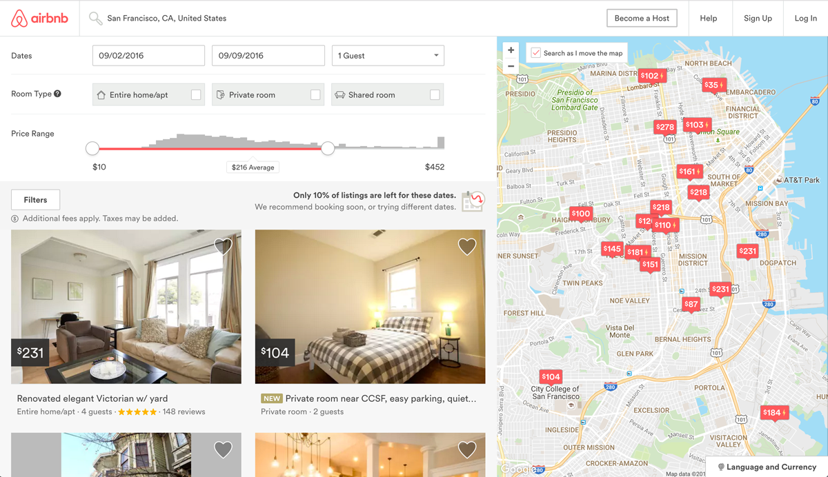
Airbnb Search Results
Airbnb搜索结果
As hosts, if we try to charge above market price then renters will select more affordable alternatives. If we set our nightly rent price too low, we’ll miss out on potential revenue.
作为房东,如果我们试图以高于市场价的价格收费,那么租房者将选择更实惠的替代方案。 如果我们将每晚租金定得太低,我们将错过潜在的收入。
One strategy we could use is to:
我们可以使用的一种策略是:
- Find a few listings that are similar to ours,
- Average the listed price for the ones most similar to ours,
- Set our listing price to this calculated average price.
- 找到一些与我们相似的清单,
- 平均与我们最相似的商品的标价,
- 将我们的挂牌价设为此计算出的平ASP格。
We’re going to build a machine learning model to automate this process using a technique called k-nearest neighbors.
我们将使用称为k最近邻居的技术来构建机器学习模型,以自动执行此过程。
First, let’s introduce the data set we’ll be working with.
首先,让我们介绍将要使用的数据集。
我们的Airbnb数据 (Our Airbnb Data)
While Airbnb doesn’t release any data on the listings in their marketplace, a separate group named Inside Airbnb has extracted data on a sample of the listings for many of the major cities on the website. In this post, we’ll be working with their data set from October 3, 2015 on the listings from Washington, D.C., the capital of the United States. Here’s a direct link to that data set. Each row in the data set is a specific listing that’s available for renting on Airbnb in the Washington, D.C. area
尽管Airbnb不会在其市场上发布有关房源的任何数据,但一个名为Inside Airbnb的独立小组已从网站上许多主要城市的房源样本中提取了数据。 在这篇文章中,我们将使用他们从2015年10月3日起在美国首都华盛顿特区上市的数据集。 这是该数据集的直接链接 。 数据集中的每一行都是一个特定的清单,可供在华盛顿特区的Airbnb上租用。
To make the data set less cumbersome to work with, we’ve removed many of the columns in the original data set and renamed the file to dc_airbnb.csv. Here are some of the more important columns:
为了减少使用数据集的麻烦,我们删除了原始数据集中的许多列,并将文件重命名为dc_airbnb.csv 。 以下是一些较重要的列:
accommodates: the number of guests the rental can accommodatebedrooms: number of bedrooms included in the rentalbathrooms: number of bathrooms included in the rentalbeds: number of beds included in the rentalprice: nightly price for the rentalminimum_nights: minimum number of nights a guest can stay for the rentalmaximum_nights: maximum number of nights a guest can stay for the rentalnumber_of_reviews: number of reviews that previous guests have left
accommodates人数:租金可容纳的客人人数bedrooms:租金中包括的bedrooms数bathrooms:租金中包含的bathrooms数量beds:租金中包含的beds数price:每晚租金minimum_nights:客人可以租用的最少住宿天数maximum_nights:客人可以租用的最大住宿天数number_of_reviews:先前访客留下的评论数
We’ll read the data set into pandas, print its size and view the first few rows.
我们将把数据集读入熊猫,打印其大小并查看前几行。
import import pandas pandas as as pdpddc_listings dc_listings = = pdpd .. read_csvread_csv (( 'dc_airbnb.csv''dc_airbnb.csv' )
)
printprint (( dc_listingsdc_listings .. shapeshape ))dc_listingsdc_listings .. headhead ()
()
(3723, 19)
| host_response_rate | host_response_rate | host_acceptance_rate | host_acceptance_rate | host_listings_count | host_listings_count | accommodates | 容纳 | room_type | 房型 | bedrooms | 卧室 | bathrooms | 浴室 | beds | 床 | price | 价钱 | cleaning_fee | 清洁费 | security_deposit | security_deposit | minimum_nights | minimum_nights | maximum_nights | maximum_nights | number_of_reviews | 评论数 | latitude | 纬度 | longitude | 经度 | city | 市 | zipcode | 邮政编码 | state | 州 | ||
|---|---|---|---|---|---|---|---|---|---|---|---|---|---|---|---|---|---|---|---|---|---|---|---|---|---|---|---|---|---|---|---|---|---|---|---|---|---|---|---|
| 0 | 0 | 92% | 92% | 91% | 91% | 26 | 26 | 4 | 4 | Entire home/apt | 整套房子/公寓 | 1.0 | 1.0 | 1.0 | 1.0 | 2.0 | 2.0 | $160.00 | $ 160.00 | $115.00 | $ 115.00 | $100.00 | $ 100.00 | 1 | 1个 | 1125 | 1125 | 0 | 0 | 38.890046 | 38.890046 | -77.002808 | -77.002808 | Washington | 华盛顿州 | 20003 | 20003 | DC | 直流电 |
| 1 | 1个 | 90% | 90% | 100% | 100% | 1 | 1个 | 6 | 6 | Entire home/apt | 整套房子/公寓 | 3.0 | 3.0 | 3.0 | 3.0 | 3.0 | 3.0 | $350.00 | $ 350.00 | $100.00 | $ 100.00 | NaN | N | 2 | 2 | 30 | 30 | 65 | 65 | 38.880413 | 38.880413 | -76.990485 | -76.990485 | Washington | 华盛顿州 | 20003 | 20003 | DC | 直流电 |
| 2 | 2 | 90% | 90% | 100% | 100% | 2 | 2 | 1 | 1个 | Private room | 私人房间 | 1.0 | 1.0 | 2.0 | 2.0 | 1.0 | 1.0 | $50.00 | $ 50.00 | NaN | N | NaN | N | 2 | 2 | 1125 | 1125 | 1 | 1个 | 38.955291 | 38.955291 | -76.986006 | -76.986006 | Hyattsville | Hyattsville | 20782 | 20782 | MD | 医学博士 |
| 3 | 3 | 100% | 100% | NaN | N | 1 | 1个 | 2 | 2 | Private room | 私人房间 | 1.0 | 1.0 | 1.0 | 1.0 | 1.0 | 1.0 | $95.00 | $ 95.00 | NaN | N | NaN | N | 1 | 1个 | 1125 | 1125 | 0 | 0 | 38.872134 | 38.872134 | -77.019639 | -77.019639 | Washington | 华盛顿州 | 20024 | 20024 | DC | 直流电 |
| 4 | 4 | 92% | 92% | 67% | 67% | 1 | 1个 | 4 | 4 | Entire home/apt | 整套房子/公寓 | 1.0 | 1.0 | 1.0 | 1.0 | 1.0 | 1.0 | $50.00 | $ 50.00 | $15.00 | $ 15.00 | $450.00 | $ 450.00 | 7 | 7 | 1125 | 1125 | 0 | 0 | 38.996382 | 38.996382 | -77.041541 | -77.041541 | Silver Spring | 银泉 | 20910 | 20910 | MD | 医学博士 |
K最近邻算法 (The K-nearest neighbors algorithm)
The K-nearest neighbors (knn) algorithm is very similar to the three step process we outlined earlier to compare our listing to similar listings and take the average price. Let’s look at it in some more detail.
K最近邻居(knn)算法与我们之前概述的将清单与相似清单进行比较并采用平ASP格的三步过程非常相似。 让我们更详细地看一下。
First, we select the number of similar listings, k, that we want to compare with.
首先,我们选择要比较的相似列表的数量k 。
Next, we need to calculate how similar each listing is to ours using a similarity metric.
接下来,我们需要使用相似度指标来计算每个列表与我们的相似度。
Then we rank each listing using our similarity metric and select the first k listings.
然后,我们使用相似性指标对每个列表进行排名,然后选择前k列表。
Finally, we calculate the mean price for the k similar listings, and use that as our list price.
最后,我们计算k类似列表的平ASP格,并将其用作我们的定价。
Let’s start by defining what similarity metric we’re going to use. Then, we’ll implement the k-nearest neighbors algorithm and use it to suggest a price for a new, unpriced listing.
让我们开始定义要使用的相似性指标。 然后,我们将实现k最近邻居算法,并使用该算法为新的未定价列表建议价格。
For the purposes of this tutorial we’re going to use a fixed k value of 5, but once you become familiar with the workflow around the algorithm you can experiment with this value to see if you get better results with lower or higher k values.
出于本教程的目的,我们将使用固定的k值5 ,但是一旦您熟悉算法周围的工作流程,就可以尝试使用该值来查看使用较低或较高k值可获得更好的结果。
When trying to predict a continuous value, like price, the main similarity metric that’s used is Euclidean distance. Here’s the general formula for Euclidean distance:
在尝试预测连续价格(例如价格)时,使用的主要相似性指标是欧几里德距离 。 这是欧几里得距离的一般公式:
where $ q_1 $ to $ q_n $ represent the feature values for one observation and $ p_1 $ to $ p_n $ represent the feature values for the other observation.
其中$ q_1 $到$ q_n $代表一个观测值的特征值,$ p_1 $到$ p_n $代表另一观测值的特征值。
建立一个简单的knn模型 (Building a simple knn model)
Let’s start by simplifying things a little, and looking at just one column. Here’s the formula for just one feature.
让我们首先简化一些事情,然后只看一列。 这是仅一项功能的公式。
The square root and the squared power cancel and the formula simplifies to:
平方根和平方幂相抵消,公式简化为:
or expressed in words, the absolute value of the difference between the observation and the data point we want to predict for the feature we’re using.
或用文字表示,即观测值与我们要为所使用功能预测的数据点之间的差的绝对值 。
The living space that we want to rent can accommodate three people. Let’s first calculate the distance, using just the accommodates feature, between the first living space in the dataset and our own.
我们要出租的居住空间可以容纳三个人。 首先,仅使用accommodates功能,计算数据集中第一个居住空间与我们自己之间的距离。
We’ll use the NumPy function np.abs() to easily calculate the absolute value.
我们将使用NumPy函数np.abs()轻松计算绝对值。
The smallest possible Euclidian distance is zero, which would mean the observation we are comparing to is identical to ours, but in isolation the value doesn’t mean much unless we know how it compares to other values.
欧几里得距离的最小可能值为零,这意味着我们正在比较的观测值与我们的观测值相同,但是孤立地讲,该值的意义并不大,除非我们知道它与其他值的比较方式。
Let’s calculate the Euclidean distance for each observation in our data set, and look at the range of values we have using pd.value_counts().
让我们为数据集中的每个观测值计算欧几里得距离,并使用pd.value_counts()查看我们拥有的值范围。
dc_listingsdc_listings [[ 'distance''distance' ] ] = = npnp .. absabs (( dc_listingsdc_listings .. accommodates accommodates - - our_acc_valueour_acc_value )
)
dc_listingsdc_listings .. distancedistance .. value_countsvalue_counts ()() .. sort_indexsort_index ()
()
0      461
1     2294
2      503
3      279
4       35
5       73
6       17
7       22
8        7
9       12
10       2
11       4
12       6
13       8
Name: distance, dtype: int64
There are 461 listings that have a distance of 0, or accommodate the same number of people as our listing.
有461个距离为0房源,或可容纳的人数与我们的房源相同。
If we just used the first five values with a distance of 0, our predictions would be biased to the existing ordering of the data set.
如果仅使用距离为0的前五个值,则我们的预测将偏向于数据集的现有排序。
Instead, we’ll randomize the ordering of the observations and then select the first five rows with a distance of 0.
相反,我们将随机化观察的顺序,然后选择距离为0的前五行。
We’re going to use DataFrame.sample() to randomize the rows. This method is usually used to select a random fraction of the dataframe, but we’ll tell it to randomly select 100%, which will randomly shuffle the rows for us.
我们将使用DataFrame.sample()将行随机化。 此方法通常用于选择数据帧的随机部分,但是我们将告诉它随机选择100%,这将为我们随机地洗排行。
We’ll also use the random_state parameter which just gives us a reproducible random order so you can follow along and get the same results.
我们还将使用random_state参数,该参数只是为我们提供了可重现的随机顺序,因此您可以沿用并获得相同的结果。
2645     $75.00
2825    $120.00
2145     $90.00
2541     $50.00
3349    $105.00
Name: price, dtype: object
Before we can take the average of our prices, you’ll notice that our price column has the object type, due to the fact that the prices have dollar signs and commas (our sample above doesn’t show the commas because all the values are less than $1000).
在我们取平ASP格之前,您会注意到我们的价格列具有object类型,这是因为价格具有美元符号和逗号(我们上面的示例未显示逗号,因为所有值都是少于$ 1000)。
Let’s clean this column by removing these characters and converting it to a float type, before calculating the mean of the first five values.
在计算前五个值的平均值之前,让我们通过删除这些字符并将其转换为float类型来清理此列。
We’ll use pandas’ Series.str.replace() to remove the stray characters and pass the regular expression $|, which will match $ or ,.
我们将使用大熊猫Series.str.replace()以去除杂散字符,并通过正则表达式$|,这将匹配$或, 。
dc_listingsdc_listings [[ 'price''price' ] ] = = dc_listingsdc_listings .. priceprice .. strstr .. replacereplace (( "$|,""$|," ,, '''' )) .. astypeastype (( floatfloat ))mean_price mean_price = = dc_listingsdc_listings .. priceprice .. ilociloc [:[: 55 ]] .. meanmean ()
()
mean_price
mean_price
We’ve now made our first prediction — our simple knn model told us that when we’re using just the accommodates feature to make predictions of our listing that accommodates three people, we should list our apartment for $88.00.
现在,我们已经做出了第一个预测-我们的简单knn模型告诉我们,当我们仅使用accommodates容纳人数功能来预测可容纳三个人的房源时,我们应该以$ 88.00的价格列出我们的公寓。
The problem is, we don’t have any way to know how accurate our model is, which makes it impossible to optimize and improve.
问题是,我们无法知道模型的准确性,因此无法进行优化和改善。
评估我们的模型 (Evaluating our model)
A simple way to test the quality of your model is to:
测试模型质量的一种简单方法是:
- Split the dataset into 2 partitions:
- The training set: contains the majority of the rows (75%)
- The test set: contains the remaining minority of the rows (25%)
- Use the rows in the training set to predict the
pricevalue for the rows in the test set - Compare the predicted values with the actual
pricevalues in the test set to see how accurate the predicted values were.
- 将数据集分为2个分区:
- 训练集:包含大多数行(75%)
- 测试集:包含剩余的少数行(25%)
- 使用训练集中的行来预测测试集中的行的
price值 - 将预测值与测试集中的实际
price值进行比较,以查看预测值的准确性。
We’re going to split the 3,723 rows of our data set into two: train_df and test_df in a 75%-25% split.
我们将把3,723行数据集分为两部分: train_df和test_df ,分为75%-25%。
Splitting into train and test dataframes
分为训练和测试数据帧
We’ll also remove the column we added earlier when we created our first model.
在创建第一个模型时,我们还将删除之前添加的列。
To make things easier for ourselves while we look at metrics, we’ll combine the simple model we made earlier into a function. We won’t need to worry about randomizing the rows, since they’re still randomized from earlier.
为了使我们在查看指标时更加轻松自如,我们将把之前制作的简单模型组合到一个函数中。 我们不必担心对行进行随机化,因为它们仍是较早前随机化的。
def def predict_pricepredict_price (( new_listing_valuenew_listing_value ,, feature_columnfeature_column ):):temp_df temp_df = = train_dftrain_dftemp_dftemp_df [[ 'distance''distance' ] ] = = npnp .. absabs (( dc_listingsdc_listings [[ feature_columnfeature_column ] ] - - new_listing_valuenew_listing_value ))temp_df temp_df = = temp_dftemp_df .. sort_valuessort_values (( 'distance''distance' ))knn_5 knn_5 = = temp_dftemp_df .. priceprice .. ilociloc [:[: 55 ]]predicted_price predicted_price = = knn_5knn_5 .. meanmean ()()returnreturn (( predicted_pricepredicted_price )
)
We can now use this function to predict values for our test dataset using the accommodates column.
现在,我们可以使用此功能使用accommodates栏来预测测试数据集的值。
使用RMSE评估我们的模型 (Using RMSE to evaluate our model)
For many prediction tasks, we want to penalize predicted values that are further away from the actual value much more than those that are closer to the actual value.
对于许多预测任务,我们要对远离实际值的预测值的惩罚要远大于接近实际值的预测值。
We can instead take the mean of the squared error values, which is called the root mean squared error (RMSE).
相反,我们可以取平方误差值的平均值,这称为均方根误差 (RMSE)。
Here’s the formula for RMSE:
这是RMSE的公式:
where n represents the number of rows in the test set.
其中, n表示测试集中的行数。
This formular might look overwhelming at first, but all we’re doing is:
最初,此公式编制者可能看起来不知所措,但我们要做的只是:
- Taking the difference between each predicted value and the actual value (or error),
- Squaring this difference (square),
- Taking the mean of all the squared differences (mean), and
- Taking the square root of that mean (root).
- 取每个预测值与实际值(或误差)之差,
- 平方这个差(平方),
- 取所有平方差的平均值(均值),然后
- 取均值的平方根(根)。
Hence, reading from bottom to top: root mean squared error.
因此,从下往上读取:均方根误差。
Let’s calculate the RMSE value for the predictions we made on the test set.
让我们为测试集上的预测计算RMSE值。
test_dftest_df [[ 'squared_error''squared_error' ] ] = = (( test_dftest_df [[ 'predicted_price''predicted_price' ] ] - - test_dftest_df [[ 'price''price' ])]) **** (( 22 )
)
mse mse = = test_dftest_df [[ 'squared_error''squared_error' ]] .. meanmean ()
()
rmse rmse = = mse mse ** ** (( 11 // 22 )
)
rmse
rmse
212.98927967051529
Our RMSE is about $213. One of the handy things about RMSE is that because we square and then take the square-root, the units for RMSE are the same as the value we are predicting, which makes it easy to understand the scale of our error.
RMSE约为213美元。 关于RMSE的方便事项之一是,因为我们先平方然后取平方根,所以RMSE的单位与我们预测的值相同,这使我们易于理解错误的范围。
比较不同型号 (Comparing different models)
With an error metric that we can use to see the accuracy of our model, let’s create some predictions using different columns and look at how our error varies.
借助误差度量标准,我们可以用来查看模型的准确性,让我们使用不同的列创建一些预测,并查看误差的变化情况。
RMSE for the accommodates column: 212.9892796705153
RMSE for the bedrooms column: 216.49048609414766
RMSE for the bathrooms column: 216.89419042215704
RMSE for the number_of_reviews column: 240.2152831433485
You can see that the best model of the four that we trained is the one using the accomodates column, however the error rates we’re getting are quite high relative to the range of prices of the listing in our data set.
您可以看到,我们训练的四个模型中最好的模型是使用accomodates栏的模型,但是相对于数据集中列表的价格范围,我们得到的错误率非常高。
So far, we’ve been training our model with only one feature, which is known as a univariate model. For more accuracy, we can use multiple features, which is known as a multivariate model.
到目前为止,我们仅使用一种功能(称为单变量模型)来训练模型。 为了获得更高的准确性,我们可以使用多个功能,称为多元模型。
We’re going to read in a cleaned version of this data set so that we can focus on evaluating the models. In our cleaned data set:
我们将阅读此数据集的完整版本,以便我们可以专注于评估模型。 在我们清理的数据集中:
- All columns have been converted to numeric values, since we can’t calculate the Euclidean distance of a value with non-numeric characters.
- Non numeric columns have been removed for simplicity.
- Any listings with missing values have been removed.
- We have normalized the columns which will give us more accurate results.
- 所有列均已转换为数字值,因为我们无法计算具有非数字字符的值的欧式距离。
- 为简单起见,非数字列已被删除。
- 缺少值的所有列表均已删除。
- 我们对列进行了归一化 ,这将为我们提供更准确的结果。
If you’d like to read more about data cleaning and preparing data for machine learning, you can read the excellent post Preparing and Cleaning Data for Machine Learning.
如果您想了解有关数据清理和为机器学习准备数据的更多信息,可以阅读出色的文章《 为机器学习准备和清理数据》 。
Let’s read in this cleaned version, which is called dc_airbnb.normalized.csv, and preview the first few rows:
让我们阅读这个干净的版本dc_airbnb.normalized.csv ,并预览前几行:
normalized_listings normalized_listings = = pdpd .. read_csvread_csv (( 'dc_airbnb_normalized.csv''dc_airbnb_normalized.csv' )
)
printprint (( normalized_listingsnormalized_listings .. shapeshape )
)
normalized_listingsnormalized_listings .. headhead ()
()
| accommodates | 容纳 | bedrooms | 卧室 | bathrooms | 浴室 | beds | 床 | price | 价钱 | minimum_nights | minimum_nights | maximum_nights | maximum_nights | number_of_reviews | 评论数 | ||
|---|---|---|---|---|---|---|---|---|---|---|---|---|---|---|---|---|---|
| 0 | 0 | -0.596544 | -0.596544 | -0.249467 | -0.249467 | -0.439151 | -0.439151 | -0.546858 | -0.546858 | 125.0 | 125.0 | -0.341375 | -0.341375 | -0.016604 | -0.016604 | 4.579650 | 4.579650 |
| 1 | 1个 | -0.596544 | -0.596544 | -0.249467 | -0.249467 | 0.412923 | 0.412923 | -0.546858 | -0.546858 | 85.0 | 85.0 | -0.341375 | -0.341375 | -0.016603 | -0.016603 | 1.159275 | 1.159275 |
| 2 | 2 | -1.095499 | -1.095499 | -0.249467 | -0.249467 | -1.291226 | -1.291226 | -0.546858 | -0.546858 | 50.0 | 50.0 | -0.341375 | -0.341375 | -0.016573 | -0.016573 | -0.482505 | -0.482505 |
| 3 | 3 | -0.596544 | -0.596544 | -0.249467 | -0.249467 | -0.439151 | -0.439151 | -0.546858 | -0.546858 | 209.0 | 209.0 | 0.487635 | 0.487635 | -0.016584 | -0.016584 | -0.448301 | -0.448301 |
| 4 | 4 | 4.393004 | 4.393004 | 4.507903 | 4.507903 | 1.264998 | 1.264998 | 2.829956 | 2.829956 | 215.0 | 215.0 | -0.065038 | -0.065038 | -0.016553 | -0.016553 | 0.646219 | 0.646219 |
We’ll then randomize the rows and split it into a train and test dataset.
然后,我们将随机化行,并将其拆分为训练和测试数据集。
计算具有多个特征的欧几里得距离 (Calculating Euclidean distance with multiple features)
Let’s remind ourselves what the original Euclidean distance equation looked like again:
让我们提醒自己原始的欧几里得距离方程又是什么样子:
We’re going to start by building a model that uses the accommodates and bathrooms attributes. For this case, our Euclidean equation would look like:
我们将从建立一个使用可accommodates和bathrooms属性的模型开始。 对于这种情况,我们的欧几里得方程如下所示:
To find the distance between two living spaces, we need to calculate the squared difference between both accommodates values, the squared difference between both bathrooms values, add them together, and then take the square root of the resulting sum. Here’s what the Euclidean distance between the first two rows in normalized_listings looks like:
为了找到两个居住空间之间的距离,我们需要计算两个accommodates值之间的平方差,两个bathrooms值之间的平方差,将它们相加,然后取所得总和的平方根。 这是normalized_listings前两行之间的欧几里得距离:
So far, we’ve been calculating Euclidean distance ourselves by writing the logic for the equation ourselves. We can instead use the distance.euclidean() function from scipy.spatial, which takes in two vectors as the parameters and calculates the Euclidean distance between them. The euclidean() function expects:
到目前为止,我们已经通过自己编写方程的逻辑来自己计算欧几里得距离。 我们可以改用scipy.spatial的distance.euclidean()函数 ,该函数接受两个向量作为参数并计算它们之间的欧几里得距离。 euclidean()函数期望:
- both of the vectors to be represented using a list-like object (Python list, NumPy array, or pandas Series)
- both of the vectors must be 1-dimensional and have the same number of elements
- 这两个向量都将使用类似列表的对象(Python列表,NumPy数组或pandas系列)来表示
- 两个向量都必须是一维的并且具有相同数量的元素
Let’s use the euclidean() function to calculate the Euclidean distance between the first and fifth rows in our dataset to practice.
让我们使用euclidean()函数来计算要练习的数据集中第一行和第五行之间的欧几里得距离。
from from scipy.spatial scipy.spatial import import distancedistancefirst_listing first_listing = = normalized_listingsnormalized_listings .. ilociloc [[ 00 ][[][[ 'accommodates''accommodates' , , 'bathrooms''bathrooms' ]]
]]
fifth_listing fifth_listing = = normalized_listingsnormalized_listings .. ilociloc [[ 2020 ][[][[ 'accommodates''accommodates' , , 'bathrooms''bathrooms' ]]
]]
first_fifth_distance first_fifth_distance = = distancedistance .. euclideaneuclidean (( first_listingfirst_listing , , fifth_listingfifth_listing )
)
first_fifth_distance
first_fifth_distance
0.9979095531766813
创建多元KNN模型 (Creating a multivariate KNN model)
We can extend our previous function to use two features and our whole data set. Instead of distance.euclidean(), we’re doing to use distance.cdist() since it allows us to pass multiple rows at once. The cdist() method can be used to calcuate distance using a variety of methods, but it defaults to Euclidean.
我们可以扩展先前的功能以使用两个功能和整个数据集。 我们正在使用distance.cdist()而不是distance.euclidean() ,因为它允许我们一次传递多行。 cdist()方法可用于通过多种方法计算距离,但默认为Euclidean。
122.702007943
You can see that our RMSE improved from 212 to 122 when using two features instead of just accommodates.
您可以看到,使用两个功能而不是仅accommodates两个功能时,我们的RMSE从212提高到122。
We’ve been writing functions from scratch to train the k-nearest neighbor models. While this is helpful to understand how the mechanics work, you can be more productive and iterate quicker by using a library that handles most of the implementation.
我们一直在从头开始编写函数,以训练k最近邻模型。 虽然这有助于理解机制的工作原理,但通过使用处理大多数实现的库,您可以提高生产率并加快迭代速度。
Scikit-learn is the most popular machine learning library in Python. Scikit-learn contains functions for all of the major machine learning algorithms and a simple, unified workflow. Both of these properties allow data scientists to be incredibly productive when training and testing different models on a new dataset.
Scikit-learn是Python中最受欢迎的机器学习库。 Scikit-learn包含所有主要机器学习算法的功能以及简单,统一的工作流程。 这两个属性使数据科学家在新数据集上训练和测试不同模型时,生产力异常提高。
The scikit-learn workflow consists of four main steps:
scikit-learn工作流程包括四个主要步骤:
- Instantiate the specific machine learning model you want to use.
- Fit the model to the training data.
- Use the model to make predictions.
- Evaluate the accuracy of the predictions.
- 实例化您要使用的特定机器学习模型。
- 使模型适合训练数据。
- 使用模型进行预测。
- 评估预测的准确性。
Each model in scikit-learn is implemented as a separate class and the first step is to identify the class we want to create an instance of. In our case, we want to use the KNeighborsRegressor class.Any model that helps us predict numerical values, like listing price in our case, is known as a regression model. The other main class of machine learning models is called classification, where we’re trying to predict a label from a fixed set of labels (e.g. blood type or gender). The word regressor from the class name KNeighborsRegressor refers to the regression model class that we just discussed.
scikit-learn中的每个模型都是作为一个单独的类实现的,第一步是识别我们要为其创建实例的类。 在本例中,我们要使用KNeighborsRegressor类 。任何可以帮助我们预测数值的模型(例如本例中的挂牌价)都称为回归模型。 机器学习模型的另一个主要类别称为分类 ,其中我们试图根据一组固定的标签(例如血型或性别)来预测标签。 从类名称中的单词回归 KNeighborsRegressor指的是我们刚才讨论的回归模型类。
Scikit-learn uses a similar object-oriented style to Matplotlib and you need to instantiate an empty model first by calling the constructor.
Scikit-learn使用与Matplotlib类似的面向对象样式,您需要首先通过调用构造函数实例化一个空模型。
from from sklearn.neighbors sklearn.neighbors import import KNeighborsRegressor
KNeighborsRegressor
knn knn = = KNeighborsRegressorKNeighborsRegressor ()
()
If you refer to the documentation, you’ll notice that by default:
如果您参考文档 ,则默认情况下您会注意到:
n_neighbors: the number of neighbors, is set to5algorithm: for computing nearest neighbors, is set toautop: set to2, corresponding to Euclidean distance
n_neighbors:邻居数,设置为5algorithm:用于计算最近的邻居,设置为autop:设置为2,对应于欧几里得距离
Let’s set the algorithm parameter to brute and leave the n_neighbors value as 5, which matches the manual implementation we built.
让我们将algorithm参数设置为brute并将n_neighbors值保留为5 ,这与我们构建的手动实现相匹配。
Now, we can fit the model to the data using the fit method. For all models, the fit method takes in two required parameters:
现在,我们可以使用fit方法使模型适合数据。 对于所有模型, fit方法采用两个必需的参数:
- matrix-like object, containing the feature columns we want to use from the training set.
- list-like object, containing correct target values.
- 类矩阵对象,包含我们要在训练集中使用的特征列。
- 类列表对象,包含正确的目标值。
Matrix-like object means that the method is flexible in the input and either a Dataframe or a NumPy 2D array of values is accepted. This means you can select the columns you want to use from the Dataframe and use that as the first parameter to the fit method.
类矩阵的对象意味着该方法在输入中很灵活,并且可以接受Dataframe或NumPy 2D值数组。 这意味着您可以从数据框中选择要使用的列,并将其用作fit方法的第一个参数。
If you recall from earlier, all of the following are acceptable list-like objects:
如果您回想起以前,以下所有都是可接受的类似列表的对象:
- NumPy array.
- Python list.
- pandas Series object (e.g. when selecting a column).
- NumPy数组。
- Python列表。
- 熊猫系列对象(例如,选择列时)。
You can select the target column from the Dataframe and use that as the second parameter to the fit method:
您可以从数据框选择目标列,并将其用作fit方法的第二个参数:
knnknn .. fitfit (( train_featurestrain_features , , train_targettrain_target )
)
When the fit() method is called, scikit-learn stores the training data we specified within the KNearestNeighbors instance (knn). If you try passing in data containing missing values or non-numerical values into the fit method, scikit-learn will return an error. Scikit-learn contains many such features that help prevent us from making common mistakes.
调用fit()方法时,scikit-learn将在KNearestNeighbors实例( knn )中指定的训练数据存储。 如果您尝试将包含缺少值或非数字值的数据传递到fit方法中,则scikit-learn将返回错误。 Scikit学习包含许多此类功能,有助于防止我们犯常见错误。
Now that we specified the training data we want used to make predictions, we can use the predict method to make predictions on the test set. The predict method has only one required parameter:
现在我们指定了要用于预测的训练数据,我们可以使用预测方法对测试集进行预测。 predict方法只有一个必需的参数:
- matrix-like object, containing the feature columns from the dataset we want to make predictions on
- 类矩阵对象,包含我们要对其进行预测的数据集中的特征列
The number of feature columns you use during both training and testing need to match or scikit-learn will return an error:
您在培训和测试期间需要匹配或scikit-learn使用的功能列数将返回错误:
The predict() method returns a NumPy array containing the predicted price values for the test set. You now have everything you need to practice the entire scikit-learn workflow.
predict()方法返回一个NumPy数组,其中包含测试集的预测price值。 现在,您拥有了练习整个scikit-learn工作流程所需的一切。
knnknn .. fitfit (( norm_train_dfnorm_train_df [[ colscols ], ], norm_train_dfnorm_train_df [[ 'price''price' ])
])
two_features_predictions two_features_predictions = = knnknn .. predictpredict (( norm_test_dfnorm_test_df [[ colscols ])
])
使用Scikit-Learn计算MSE (Calculating MSE using Scikit-Learn)
Up until this point we have been calculating RMSE values manually, both using NumPy and SciPy functions to assist us. Alternatively, we can instead use the sklearn.metrics.mean_squared_error function(). Once you become familiar with the different machine learning concepts, unifying your workflow using scikit-learn helps save you a lot of time and helps you avoid mistakes.
到目前为止,我们一直在使用NumPy和SciPy函数来协助我们手动计算RMSE值。 或者,我们可以改用sklearn.metrics.mean_squared_error function() 。 一旦您熟悉了不同的机器学习概念,使用scikit-learn统一工作流程将帮助您节省大量时间并避免出错。
The mean_squared_error() function takes in two inputs:
mean_squared_error()函数接受两个输入:
- A list-like object, representing the true values.
- A second list-like object, representing the predicted values using the model.
- 类似于列表的对象,代表真实值。
- 第二个类似列表的对象,代表使用模型的预测值。
124.834722314
Not only is this much simpler from a syntax perspective, but it also takes less time for the model to run as scikit-learn has been heavily optimized for speed.
从语法的角度来看,这不仅简单得多,而且由于scikit-learn已针对速度进行了大幅优化,因此运行模型所需的时间更少。
You’ll notice that our RMSE is a little different from our manually implemented algorithm — this is likely due to both differences in the randomization and slight differences in implementation between our ‘manual’ KNN algorithm and the scikit-learn version.
您会注意到,我们的RMSE与手动实现的算法略有不同-这可能是由于随机差异以及我们的“手动” KNN算法和scikit-learn版本之间在实现上的细微差异。
使用更多功能 (Using more features)
One of the best things about scikit-learn is that it allows us to iterate quicker.
scikit-learn最好的事情之一是它使我们可以更快地进行迭代。
Let’s see this in action, by creating a model which uses four features instead of two and see if that improves our results.
让我们通过创建一个使用四个特征而不是两个特征的模型来看看实际情况,看看是否可以改善我们的结果。
knn knn = = KNeighborsRegressorKNeighborsRegressor (( algorithmalgorithm == 'brute''brute' ))cols cols = = [[ 'accommodates''accommodates' ,, 'bedrooms''bedrooms' ,, 'bathrooms''bathrooms' ,, 'beds''beds' ]]knnknn .. fitfit (( norm_train_dfnorm_train_df [[ colscols ], ], norm_train_dfnorm_train_df [[ 'price''price' ])
])
four_features_predictions four_features_predictions = = knnknn .. predictpredict (( norm_test_dfnorm_test_df [[ colscols ])
])
four_features_mse four_features_mse = = mean_squared_errormean_squared_error (( norm_test_dfnorm_test_df [[ 'price''price' ], ], four_features_predictionsfour_features_predictions )
)
four_features_rmse four_features_rmse = = four_features_mse four_features_mse ** ** (( 11 // 22 )
)
four_features_rmse
four_features_rmse
120.92729413345498
In this case, our error went down slightly, but it may not always do so as you add features.
在这种情况下,我们的错误会略有下降,但是在您添加功能时可能并不总是如此。
This is an important thing to be aware of – more features does not necessarily make an accurate model, since adding a feature that is not an accurate predictor of your target variable adds ‘noise’ to your model.
注意这一点很重要-更多功能不一定能形成准确的模型,因为添加的功能不能准确预测目标变量,因此会给模型增加“噪音”。
摘要 (Summary)
Let’s take a look at what we’ve learned:
让我们看看我们学到了什么:
- We learned what machine learning is.
- We learned about the k-nearest neighbors algorithm, and built a univariate model (only one feature) from scratch and used it to make predictions.
- We learned that RMSE can be used to calculate the error of our models, which we can then use to iterate and try and improve our predictions.
- We then created a multivariate (more than one feature) model from scratch and used that to make predictions.
- Finally, we learned about the scikit-learn library, and used the
KNeighborsRegressorclass to make predictions.
- 我们了解了什么是机器学习。
- 我们了解了k近邻算法,并从头开始构建了一个单变量模型(仅一个特征),并用其进行了预测。
- 我们了解到,RMSE可用于计算模型的误差,然后可用于迭代和尝试并改进我们的预测。
- 然后,我们从头创建了一个多变量(多个功能)模型,并将其用于进行预测。
- 最后,我们了解了scikit-learn库,并使用
KNeighborsRegressor类进行了预测。
下一步 (Next Steps)
翻译自: https://www.pybloggers.com/2017/08/machine-learning-fundamentals-predicting-airbnb-prices/
airbnb机器学习模型
airbnb机器学习模型_机器学习基础:预测Airbnb价格相关推荐
- 机器学习 可视化_机器学习-可视化
机器学习 可视化 机器学习导论 (Introduction to machine learning) In the traditional hard-coded approach, we progra ...
- 机器学习:分类_机器学习基础:K最近邻居分类
机器学习:分类 In the previous stories, I had given an explanation of the program for implementation of var ...
- 基于张量机器学习模型_什么是基于模型的机器学习?
基于张量机器学习模型 About Tom: Tom Diethe is a research fellow on the SPHERE project at the University of Bri ...
- 基于三种机器学习模型的岩爆类型预测及Python实现
写在前面 由于代码较多,本文仅展示部分关键代码,需要代码文件和数据可以留言 然而,由于当时注释不及时,且时间久远,有些细节笔者也记不清了,代码仅供参考 0 引言 岩爆是深部岩土工程施工过程中常见的一种 ...
- 加载svr模型_机器学习XGBoost实战,网格搜索自动调参,对比随机森林,线性回归,SVR【完整代码(含注释)+数据集见原文链接】...
建议:阅读2020.8.7的文章,完全了解GDBT和XGBT的原理. 机器学习- XGBoost,GDBT[过程:决策树,集成学习,随机森林,GDBT,XGBT,LightGBM] 本次实践内容: 数 ...
- 深度学习的可解释性 github_机器学习模型可解释性实战-预测世界杯当场最佳
笔者在之前的一篇博客<谈谈机器学习模型的可解释性>介绍了机器学习可解释性的基本概念,那么今天我们就来看看如何具体的利用这些可解释的工具来对一个真实的模型进行可解释性的分析. 本文所有代码参 ...
- sklearn保存svm分类模型_机器学习100天-Day1601线性支持向量机分类
说明:本文依据<Sklearn 与 TensorFlow 机器学习实用指南>完成,所有版权和解释权均归作者和翻译成员所有,我只是搬运和做注解. 第五章是对支持向量机SVM的系统介绍,阐述支 ...
- 机器学习指南_机器学习项目的研究指南
机器学习指南 Machine Learning projects can be delivered in two stages. The first stage is named Research a ...
- 机器学习术语_机器学习术语神秘化。
机器学习术语 Till this day, my favorite definition of a Machine is ; something that makes work easier. At ...
最新文章
- 为了效率,扎克伯格的26张PPT
- hihoCoder 网络流四·最小路径覆盖
- TS2003基于触摸屏的应用
- Angular2学习笔记——NgModule
- 深入浅出Javascript闭包
- java传送字符到前端_javaWeb后台特殊字符怎样还原传给前端正确显示?
- 关于python3的readlines(),read()和readline()简介
- 让IE的F1帮助变成自己的
- 平面设计和网页设计的规则_从平面设计到用户界面:这是您应该知道的最重要的规则
- 移动端 uniapp 国际化一站式解决方案
- spring 源码深度解析_spring源码解析之SpringIOC源码解析(下)
- VM虚拟机安装centos6.3详细图文教程
- 制作目标在背景中具有移动效果的视频
- Dell Precision M4800 VoodooPS2Controller 键盘/触控驱动修复过程
- 27年台湾珍珠鲜奶茶品牌Sharetea将引进上海
- 安卓的第三方sdk是html,第三方SDK目录
- 接口测试-使用Postman发送请求
- Python3+Flickrapi爬取图片
- java字符串tirm方法模拟去除首尾空白字符
- java输出字符串的长度_Java格式化字串输出固定长度