Churn prediction, namely predicting clients who might want to turn down the service, is one of the most common business applications of machine learning. It is especially important for those companies providing streaming services. In this project, an event data set from a fictional music streaming company named Sparkify was analyzed. A tiny subset (128MB) of the full dataset (12GB) was first analyzed locally in Jupyter Notebook with a scalable script in Spark and the whole data set was analyzed on the AWS EMR cluster. Find the code here.

流失预测(即预测可能要拒绝服务的客户)是机器学习最常见的业务应用之一。 对于提供流媒体服务的公司而言，这一点尤其重要。 在该项目中，分析了一家虚构的音乐流媒体公司Sparkify的事件数据集。 首先在Jupyter Notebook中使用Spark中的可扩展脚本在本地对整个数据集(12GB)的一小部分(128MB)进行分析，然后在AWS EMR集群上分析整个数据集。 在此处找到代码。

资料准备 (Data preparation)

Let’s first have a look at the data. There were 286500 rows and 18 columns in the mini data set (in the big data set, there were 26259199 rows). The columns and first five rows were shown as follows.

首先让我们看一下数据。 小型数据集中有286500行和18列(在大数据集中有26259199行)。 列和前五行如下所示。

Let’s check missing values in the data set. We will find a pattern from the table below in the missing values: There was the same number of missing values in the “artist”,” length”, and the ”song” columns, and the same number of missing values in the “firstName”, “gender”, “lastName”, “location”,” registration”, and ”userAgent” columns.

让我们检查数据集中的缺失值。 我们将从下表中找到缺失值的模式：“艺术家”，“长度”和“歌曲”列中缺失值的数量相同，而“名字”中缺失值的数量相同”，“性别”，“姓氏”，“位置”，“注册”和“ userAgent”列。

If we see closer at the “userId”, whose “firstName” was missing, we will find that those “userId” was actually empty strings (in the bid data was the user with the ID 1261737), with exactly 8346 records (with 778479 rows in the bid data), which I decided to treat as missing values and deleted. This might be someone who has only visited the Sparkify website without registering.

如果我们更靠近“ userId”(缺少“ firstName”)，我们会发现这些“ userId”实际上是空字符串(在出价数据中是ID为1261737的用户)，正好有8346条记录(778778)出价数据中的所有行)，我决定将其视为缺失值并删除。 这可能是只访问了Sparkify网站但未注册的人。

After deleting the “problematic” userId, there was 255 unique users left (this number was 22277 for the big data).

删除“有问题的”用户ID后，剩下255个唯一用户(大数据该数字为22277)。

Let’s dig further on remaining missing values. As the data is event data, which means every operation of single users was recorded. I hypothesized that those missing values in the “artist” column might have an association with the certain actions (page visited) of the users, that’s why I check the visited “pages” associated with the missing “artist” and compared with the “pages” in the complete data and found that: “missing artist” is combined with all the other pages except “next song”, which means the “artist” (singer of the song) information is recorded only when a user hit “next song”.

让我们进一步研究剩余的缺失值。 由于数据是事件数据，因此意味着记录了单个用户的每项操作。 我假设“艺术家”列中的那些缺失值可能与用户的某些操作(访问的页面)相关联，这就是为什么我检查与缺失的“艺术家”相关联的访问过的“页面”并与“页面”进行比较的原因”中的完整数据，发现：“缺少歌手”与除“下一首歌”以外的所有其他页面组合在一起，这意味着仅当用户按下“下一首歌”时，“歌手”(歌曲的歌手)信息才会被记录。

If I delete those “null” artist rows, there will be no missing values anymore in the data set and unique users number in the clean data set will still be 255.

如果删除这些“空”艺术家行，则数据集中将不再缺少任何值，并且干净数据集中的唯一用户数仍为255。

After dealing with missing values, I transformed timestamp into epoch date, and simplified two categorical columns, extracting only “states” information from the “location” column and platform used by the users (marked as “agent”) from the “userAgent” column.

处理完缺失值后，我将时间戳转换为时代日期，并简化了两个分类列，仅从“位置”列和“ userAgent”列中用户使用的平台(标记为“代理”)中提取“状态”信息。

The data cleaning step is completed so far, and let’s start to explore the data and find out more information. As the final purpose is to predict churn, we need to first label the churned users (downgrade was also labeled in the same method). I used the “Cancellation Confirmation” events to define churn: those churned users who visited the “Cancellation Confirmation” page was marked as “1”, and who did not was marked as “0”. Similarly who visited page “Downgrade” at least once was marked as “1”, and who did not was marked as “0”. Now the data set with 278154 rows and columns shown below is ready for some exploratory analysis. Let’s do some comparisons between churned and stayed users.

到目前为止，数据清理步骤已经完成，让我们开始探索数据并查找更多信息。 由于最终目的是预测用户流失，因此我们需要先标记流失的用户(降级也用相同的方法标记)。 我使用“取消确认”事件来定义用户流失：那些访问“取消确认”页面的搅动用户被标记为“ 1”，而没有被标记为“ 0”的用户。 同样，至少访问过一次“降级”页面的人被标记为“ 1”，而没有访问过的人被标记为“ 0”。 现在，下面显示的具有278154行和列的数据集已准备好进行一些探索性分析。 让我们在流失用户和停留用户之间进行一些比较。

搅动和停留用户的数量，性别，级别和降级情况 (Number, gender, level, and downgrade condition of churned and stayed users)

There were 52 churned and 173 stayed users in the small data set (those numbers were 5003 and 17274 respectively for the big data), with slightly more males than females in both groups (left figure below). It seemed that among the stayed users there were more people who have downgraded their account at least once (right figure below).

在小型数据集中，有52位搅拌用户和173位常住用户(大数据分别为5003和17274)，两组中男性均比女性略多(下图)。 似乎，在留下来的用户中，有更多人至少一次降级了他们的帐户(下图右图)。

The “level” column has two values “free” and “paid”. Some users might have changed their level more than once. To check how “level” has differed between churned and stayed users, a “valid_level” column was created to record the latest level of users. As shown in the figure below, there are more paid users among the stayed users.

“级别”列具有两个值“免费”和“已付费”。 一些用户可能已多次更改其级别。 为了检查搅动和停留的用户之间的“级别”有何不同，创建了一个“ valid_level”列来记录最新的用户级别。 如下图所示，在停留的用户中有更多的付费用户。

注册天数，每天的歌曲数和每个会话的歌曲数 (Registered days, number of songs per day and number of songs per session)

The stayed users registered for more days than the churned users apparently, and the stayed users played on average more songs than the churned users both on a daily and a session base.

停留的用户注册的时间显然比搅拌的用户多，并且停留的用户在每天和会话基础上播放的歌曲平均比搅拌的用户多。

每日平均每次会话项目和平均会话持续时间 (Daily average item per session and average session duration)

As shown below, the daily average item per session was slightly higher for stayed users than churned users.

如下所示，对于留用用户，每个会话的每日平均项目要略高于搅动用户。

The average session duration was also longer for stayed users than churned users.

停留的用户的平均会话持续时间也比搅动的用户更长。

用户活动分析 (User activities analysis)

To analyze how the user activities differ between churned and stayed users, the daily average numbers of “thumbs up”, “add to playlist”, “add friend”, “roll adverts”, and” thumbs down” for each user were calculated. Those features were selected because they were the most visited pages among others (see table below).

为了分析搅动和停留用户之间的用户活动差异，计算了每个用户每天的“竖起大拇指”，“添加到播放列表”，“添加朋友”，“滚动广告”和“竖起大拇指”的平均数量。 选择这些功能是因为它们是其他页面中访问量最大的页面(请参见下表)。

As a result, churned users added fewer friends, gave less “thumbs up”, and added fewer songs into their playlists on a daily base than stayed users. While the churned users gave more “thumbs down” and rolled over more advertisements daily than stayed users.

结果，与留宿用户相比，每天搅动的用户添加更少的朋友，减少“竖起大拇指”，并且将更少的歌曲添加到他们的播放列表中。 尽管流失的用户每天比停留的用户更多地“竖起大拇指”，并滚动更多的广告。

两组用户的平台和位置 (The platform and location of two groups of users)

The platform (marked as “agent” in the table) used by users are plotted below. It appeared that the churning rates were different among the six agents. It means the platform on which the users are using Sparkify’s service might influence churn.

用户绘制的平台(表中标记为“代理”)如下图所示。 看来这六个代理商的流失率是不同的。 这意味着用户使用Sparkify服务的平台可能会影响用户流失。

Similarly, the churning rates seemed to be changing in different states (see figure below).

同样，不同国家的流失率似乎也在变化(见下图)。

特征工程 (Feature engineering)

Before fitting any model, the following columns were assembled to create the final data set df_model for modeling.

在拟合任何模型之前，将以下各列进行组装，以创建用于建模的最终数据集df_model 。

Response variable

响应变量

label: 1 for churned and 0 for not

标签：1表示搅动，0表示不搅动

Explanatory variables (categorical)

解释变量(分类)

downgraded: 1 for downgraded and 0 for not

降级：1表示降级，0表示​​不降级

gender: M for male and F for female

性别：男为男，女为男

valid_level: free or paid

valid_level：免费或付费

agent: platform used by users with five categories (windows, macintosh, iPhone, iPad, and compatible)

代理：供五类用户使用的平台(Windows，macintosh，iPhone，iPad和兼容)

Explanatory variables (numeric)

解释变量(数字)

registered_days: counted by the maximum value of “ts” (timestamp of actions) subtracted by “registration” timestamp and transformed to days

registered_days：以“ ts”(动作时间戳记)的最大值减去“ registration”时间戳记后转换为天数

avg_daily_song: average song listened on a daily base

avg_daily_song：每天平均听一首歌

songs_per_session: average songs listened per session

songs_per_session：每个会话平均听过的歌曲

avg_session: average session duration

avg_session：平均会话持续时间

friends: daily number of friends added by a user

朋友：用户每天添加的朋友数

thumbs up: daily number of thumbs up given by a user

竖起大拇指：用户每天给出的竖起大拇指的次数

thumbs down: daily number of thumbs down given by a user

大拇指朝下：用户每天给予的大拇指朝下的次数

add_playlist: daily number of “add to playlist” action

add_playlist：“添加到播放列表”操作的每日次数

roll_advert: daily number of “roll advert” action

roll_advert：“滚动广告”操作的每日次数

Categorical variables ‘gender’,’valid_level’, and ’agent’ were first transformed into indexes using the StringIndexer.

首先使用StringIndexer将分类变量“ gender”，“ valid_level”和“ agent”转换为索引。

# creating indexs for the categorical columnsindexers = [StringIndexer(inputCol=column, outputCol=column+"_index").fit(df_model) for column in ['gender','valid_level','agent'] ]pipeline = Pipeline(stages=indexers)df_r = pipeline.fit(df_model).transform(df_model)df_model = df_r.drop('gender','valid_level','agent')

And the numeric variables were first assembled into a vector using VectorAssembler and then scaled using StandardScaler.

然后，首先使用VectorAssembler将数字变量组装为向量，然后使用StandardScaler对其进行缩放。

# assembeling numeric features to create a vectorcols=['registered_days','friends','thumbs_ups','thumbs_downs','add_playlist','roll_advert',\      'daily_song','session_song','session_duration']assembler = VectorAssembler(inputCols=cols,outputCol="features")# use the transform method to transform dfdf_model = assembler.transform(df_model)# standardize numeric feature vectorstandardscaler=StandardScaler().setInputCol("features").setOutputCol("Scaled_features")df_model = standardscaler.fit(df_model).transform(df_model)

In the end, all the categorical and numeric features were combined and again transformed into a vector.

最后，将所有类别和数字特征组合在一起，然后再次转换为向量。

cols=['Scaled_features','downgraded','gender_index','valid_level_index','agent_index']assembler = VectorAssembler(inputCols=cols,outputCol='exp_features')# use the transform method to transform dfdf_model = assembler.transform(df_model)

造型 (Modeling)

As the goal was to predict a binary result (1 for churn and 0 for not), logistic regression, random forest, and gradient boosted tree classifiers were selected to fit the data set. F1 score and AUC were calculated as evaluation metrics. Because our training data was imbalanced (there were fewer churned than stayed users). And from the perspective of the company, incorrectly identifying a user who was going to churn is more costly. In this case, F1-score is a better metric than accuracy, because it provides a better measure of the incorrectly classified cases (for more information click here). AUC, on the other hand, gives us a perspective over how good the model is regarding the separability, in another word, distinguishing 1 (churn) from 0 (stay).

由于目标是预测二进制结果(流失为1，否则为0)，因此选择了逻辑回归，随机森林和梯度增强树分类器以适合数据集。 计算F1分数和AUC作为评估指标。 因为我们的训练数据不平衡(搅动的人数少于留守的使用者)。 而且从公司的角度来看，错误地标识将要流失的用户的成本更高。 在这种情况下，F1评分比准确度更好，因为它可以更好地衡量分类错误的案例(有关更多信息，请单击此处 )。 另一方面， AUC为我们提供了关于模型关于可分离性的良好程度的观点，换句话说，将1(搅动)与0(保持)区分开。

The data set was first broke into 80% of training data and 20% as a test set.

首先将数据集分为训练数据的80％和测试集的20％。

rest, validation = df_model.randomSplit([0.8, 0.2], seed=42)

逻辑回归模型 (Logistic regression model)

There were more stayed users than churned users in the whole data set, and in our training set the number of churned is 42, which represents only around 22% of total users. To solve this imbalance problem and get better prediction results, class_weights values were introduced into the model.

在整个数据集中，停留的用户多于搅动的用户，在我们的训练集中，搅动的数量为42，仅占总用户的22％。 为了解决此不平衡问题并获得更好的预测结果，将class_weights值引入模型。

A logistic regression model with weighed features was built like the following and BinaryClassificationEvaluator was used to evaluate the model.

建立具有权重特征的逻辑回归模型，如下所示，并使用BinaryClassificationEvaluator评估模型。

# Initialize logistic regression objectlr = LogisticRegression(labelCol="label", featuresCol="exp_features",weightCol="classWeights",maxIter=10)# fit the model on training setmodel = lr.fit(rest)# Score the training and testing dataset using fitted model for evaluation purposespredict_rest = model.transform(rest)predict_val = model.transform(validation)# Evaluating the LR model using BinaryClassificationEvaluatorevaluator = BinaryClassificationEvaluator(rawPredictionCol="rawPrediction",labelCol="label")#F1 scoref1_score_evaluator = MulticlassClassificationEvaluator(metricName='f1')f1_score_rest = f1_score_evaluator.evaluate(predict_rest.select(col('label'), col('prediction')))f1_score_val = f1_score_evaluator.evaluate(predict_val.select(col('label'), col('prediction')))#AUC auc_evaluator = BinaryClassificationEvaluator()roc_value_rest = auc_evaluator.evaluate(predict_rest, {auc_evaluator.metricName: "areaUnderROC"})roc_value_val = auc_evaluator.evaluate(predict_val, {auc_evaluator.metricName: "areaUnderROC"})

The scores of the logistic regression model were like the following:

逻辑回归模型的得分如下：

The F1 score on the train set is 74.38%The F1 score on the test set is 73.10%The areaUnderROC on the train set is 79.43%The areaUnderROC on the test set is 76.25%

And the feature importance is shown as the following. The feature registered days, the average number of songs listened per session, and the average session duration was negatively associated with churn, while the average number of songs listened per session and the action of downgraded was positively associated with churn. In another word, users who listen to more songs per day and downgraded at least once are more likely to churn. Whereas, the longer one session lasts and the more songs one listens per session, the less likely for this user to churn.

并且功能重要性如下所示。 该功能注册的天数，每个会话中平均听的歌曲数，平均会话持续时间与客户流失率呈负相关，而每个会话中平均听的歌曲数和降级行为与客户流失率呈正相关。 换句话说，每天听更多歌曲并且至少降级一次的用户更有可能流失。 而一个会话持续的时间越长，每个会话聆听的歌曲越多，则该用户流失的可能性就越小。

It sounds a bit irrational that, the more songs one listens per day, the more likely for him to churn. To draw a safe conclusion, I would include more samples to fit the model again. This will be the future work.

听起来有点不合理，因为每天听的歌曲越多，他流失的可能性就越大。 为了得出一个安全的结论，我将包括更多样本以再次适合模型。 这将是未来的工作。

随机森林模型 (Random forest model)

In a similar manner, a random forest model was fit into the training data, refer the original code here. And the metrics were as the following:

以类似的方式，将随机森林模型拟合到训练数据中，请在此处参考原始代码。 指标如下：

The F1 score on the train set is 90.21%The F1 score on the test set is 70.31%The areaUnderROC on the train set is 98.21%The areaUnderROC on the test set is 80.00%

There is obviously an overfitting problem. Both the F1 and AUC scores were very high for the training set and poorer in the test set. The feature importance analysis showed: Besides registered days and songs listened per day, the number of friends added, thumbs up, and thumbs down given on a daily base were the most important features regarding churn prediction. As future work, I would fit this model again on the big data set to see if adding samples will solve the overfitting problem.

显然存在过度拟合的问题。 F1和AUC分数在训练集中都非常高，而在测试集中则较差。 特征重要性分析表明：除了记录的天数和每天听的歌曲之外，每天增加的好友数，竖起大拇指和竖起大拇指都是关于流失预测的最重要特征。 在以后的工作中，我将再次将该模型适合大数据集，以查看添加样本是否可以解决过拟合问题。

梯度提升树模型 (Gradient boosted tree model)

GBT model showed a more severe overfitting problem. A suggestion for improvement will be the same as mentioned before. Try on the big data set first, if necessary do finer feature engineering or try other methods.

GBT模型显示了更严重的过度拟合问题。 改进的建议与前面提到的相同。 首先尝试大数据集，必要时进行更精细的功能设计或尝试其他方法 。

The F1 score on the train set is 99.47%The F1 score on the test set is 68.04%The areaUnderROC on the train set is 100.00%The areaUnderROC on the test set is 64.58%

超参数调整和交叉验证 (Hyperparameter tuning and cross-validation)

According to the F1 and AUC scores of all three models, I decided to pick the logistic regression model to do further hyperparameter tuning and 3-fold cross-validation.

根据这三个模型的F1和AUC分数，我决定选择逻辑回归模型进行进一步的超参数调整和3倍交叉验证。

# logistic regression model parameters tuninglrparamGrid = ParamGridBuilder() \    .addGrid(lr.elasticNetParam,[0.0, 0.1, 0.5]) \    .addGrid(lr.regParam,[0.0, 0.05, 0.1]) \    .build()

However, except for an obvious improvement in model performance on the training set. Both the F1 and AUC scores were lower on the test set. For an overfitting situation, parameter tuning was a bit tricky, and cross-validation did not help in this case to improve model performance, check the link here which might through some insight into this problem.

但是，除了训练集上的模型性能有明显改善外。 F1和AUC分数在测试集上均较低。 对于过度拟合的情况，参数调整有些棘手，在这种情况下，交叉验证无助于提高模型性能，请查看此处的链接 ，这可能会通过一些洞察力来解决此问题。

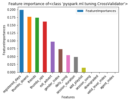
The F1 score on the train set is 87.73%The F1 score on the test set is 72.74%The areaUnderROC on the train set is 91.27%The areaUnderROC on the test set is 78.33%

Feature importance of logistic regression after parameter tuning and cross-validation showed a different pattern from before. The registered day was the most promising indicator of churn (this information might with little interest to the service provider company). Besides, the number of thumbs-ups, friends added, thumbs-downs and roll advert were the features with the highest importance.

参数调整和交叉验证后逻辑回归的特征重要性显示出与以前不同的模式。 注册日是流失率最有希望的指标(服务提供商公司可能对此信息不太感兴趣)。 此外，最重要的功能是大拇指向上，朋友添加，大拇指向下和滚动广告的数量。

结论 (Conclusion)

In this project, churn prediction was performed based on an event data set for a music streaming provider. This was basically a binary classification problem. After loading and cleaning data, I performed some exploratory analysis and provided insights on the next step of feature engineering. All together 13 explanatory features were selected and logistic regression, random forest, and gradient-boosted tree models were fitted respectively to a training data set.

在该项目中，根据针对音乐流媒体提供商的事件数据集执行了流失预测。 这基本上是一个二进制分类问题。 加载和清理数据后，我进行了一些探索性分析，并就功能设计的下一步提供了见解。 总共选择了13个解释特征，并将逻辑回归，随机森林和梯度提升树模型分别拟合到训练数据集。

The model performance was the best for the logistic regression on small data set, with an F1 score of 73.10 on the test set. The other two models were both suffered from overfitting. Hyperparameter tuning and cross-validation was not very helpful in solving overfitting, probably because of a small number of sample size. Due to time and budget limitations, the final models were not tested on the big data set. However, the completely scalable process shed a light on solving the churn prediction problem on big data with Spark on Cloud.

模型性能对于小数据集的逻辑回归最好，测试集的F1得分为73.10。 另外两个模型都过度拟合。 超参数调整和交叉验证对解决过度拟合的帮助不是很大，这可能是因为样本数量很少。 由于时间和预算的限制，最终模型未在大数据集上进行测试。 但是，完全可扩展的过程为使用Spark on Cloud解决大数据的客户流失预测问题提供了启示。

讨论区 (Discussion)

Feature engineering

特征工程

How to chose the proper explanatory features was one of the most critical steps in this task. After EDA, I simply included all the features that I created. I wanted to create more features, however, the further computation was dragged down by limited computation capacity. There are some techniques ( for example the ChiSqSelector provided by Spark ML) on feature engineering that might help in this step. The “state” column had 58 different values (100 for the big data). I tried to turn them into index values using StringIndexer and include it to the explanatory feature. However, it was not possible to build a random forest/GBTs model with indexes exceeded the maxBins (= 32), that’s why I had to exclude this feature. If it was possible to use the dummy variable of this feature, the problem could have been avoided. It was a pity that I run out of time and did not manage to do a further experiment.

如何选择适当的解释功能是此任务中最关键的步骤之一。 在EDA之后，我只包含了我创建的所有功能。 我想创建更多功能，但是，由于计算能力有限，进一步的计算被拖累了。 在要素工程上有一些技术 (例如，Spark ML提供的ChiSqSelector)可能在此步骤中有所帮助。 “状态”列具有58个不同的值(大数据为100个)。 我尝试使用StringIndexer将它们转换为索引值，并将其包含在说明功能中。 但是，无法建立索引超过maxBins(= 32)的随机森林/ GBTs模型，这就是为什么我必须排除此功能。 如果可以使用此功能的哑变量，则可以避免该问题。 遗憾的是我时间不够用，没有做进一步的实验。

Computing capacity

计算能力

Most of the time I spent on this project was “waiting” for the result. It was very frustrating that I had to stop and run the codes from the beginning over and over again due to stage errors because the cluster was running out of memory. To solve this problem, I had to separate my code into two parts (one for modeling) and the other for plotting and run them separately. And I have to reduce the number of explanatory variables that I created. It was a pity that I only managed once to run the simple version of code for the big data set on AWS cluster (refer to the code here) and had to stop because it took too much time and cost. The scores of the build models on the big data set were unfortunately not satisfying. However, the last version of codes (Sparkify_visualization and Sparkify_modeling in Github repo) should be completely scalable. The performance of models on big data set should be improved if the latest codes are to be run on the big data again.

我在这个项目上花费的大部分时间都是在“等待”结果。 令人沮丧的是，由于阶段错误，我不得不从头开始一遍又一遍地停止并运行代码，因为群集内存不足。 为了解决这个问题，我不得不将代码分成两部分(一个用于建模)，另一个用于绘图并分别运行。 而且我必须减少创建的解释变量的数量。 遗憾的是，我只为AWS集群上的大数据集运行了简单版本的代码(请参阅此处的代码)，却不得不停止，因为这花费了太多时间和成本。 不幸的是，大数据集上构建模型的分数并不令人满意。 但是，代码的最新版本(Github存储库中的Sparkify_visualization和Sparkify_modeling)应该是完全可伸缩的。 如果要在大数据上再次运行最新代码，则应提高大数据集上模型的性能。

Testing selective sampling method

测试选择性抽样方法

Because the training data set is imbalanced with more “0” labeled rows than “1”, I wanted to try if randomly selecting the same number of “0” rows as “1” rows would have improved the model performance. Due to the time limit, it will be only the work for the future.

因为训练数据集的“ 0”行比“ 1”行更多，所以我想尝试一下，如果随机选择与“ 1”行相同数量的“ 0”行可以改善模型性能。 由于时间限制，这只是未来的工作。

ps: one extra tip which might be very useful, perform “cache” on critical points to speed up the program.

ps：一个可能非常有用的额外技巧，对关键点执行“缓存”以加快程序运行速度。

Any discussion is welcome! Please reach me through LinkedIn and Github

欢迎任何讨论！ 请通过LinkedIn和Github与我联系