非线性最优化（二）——高斯牛顿法和Levengerg-Marquardt迭代

高斯牛顿法和Levengerg-Marquardt迭代都用来解决非线性最小二乘问题(nonlinear least square)。

From Wiki

The Gauss–Newton algorithm is a method used to solve non-linear least squares problems. It is a modification of Newton's method for finding a minimum of a function. Unlike Newton's method, the Gauss–Newton algorithm can only be used to minimize a sum of squared function values, but it has the advantage that second derivatives, which can be challenging to compute, are not required.

Description

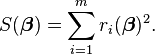
Given m functions r = (r₁, …, r_m) of n variables β = (β₁, …, β_n), with m ≥ n, the Gauss–Newton algorithm iteratively finds the minimum of the sum of squares

Starting with an initial guess for the minimum, the method proceeds by the iterations

where, if r and β are column vectors, the entries of the Jacobian matrix are

and the symbol denotes the matrix transpose.

If m = n, the iteration simplifies to

which is a direct generalization of Newton's method in one dimension.

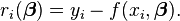
In data fitting, where the goal is to find the parameters β such that a given model function y = f(x, β) best fits some data points (x_i, y_i), the functions r_iare the residuals

Then, the Gauss-Newton method can be expressed in terms of the Jacobian J_f of the function f as

Notes

The assumption m ≥ n in the algorithm statement is necessary, as otherwise the matrix J_r^TJ_r is not invertible (rank(J_r^TJ_r)=rank(J_r))and the normal equations (Δ in the "derivation from Newton's method" part) cannot be solved (at least uniquely).

The Gauss–Newton algorithm can be derived by linearly approximating the vector of functions r_i. Using Taylor's theorem, we can write at every iteration:

with The task of finding Δ minimizing the sum of squares of the right-hand side, i.e.,

is a linear least squares problem, which can be solved explicitly, yielding the normal equations in the algorithm.

The normal equations are m linear simultaneous equations in the unknown increments, Δ. They may be solved in one step, using Cholesky decomposition, or, better, the QR factorization of J_r. For large systems, an iterative method, such as the conjugate gradient method, may be more efficient. If there is a linear dependence between columns of J_r, the iterations will fail as J_r^TJ_r becomes singular.

Derivation from Newton's method

In what follows, the Gauss–Newton algorithm will be derived from Newton's method for function optimization via an approximation. As a consequence, the rate of convergence of the Gauss–Newton algorithm can be quadratic under certain regularity conditions. In general (under weaker conditions), the convergence rate is linear.

The recurrence relation for Newton's method for minimizing a function S of parameters, , is

where g denotes the gradient vector of S and H denotes the Hessian matrix of S. Since , the gradient is given by

Elements of the Hessian are calculated by differentiating the gradient elements, , with respect to

The Gauss–Newton method is obtained by ignoring the second-order derivative terms (the second term in this expression). That is, the Hessian is approximated by

where are entries of the Jacobian J_r. The gradient and the approximate Hessian can be written in matrix notation as

These expressions are substituted into the recurrence relation above to obtain the operational equations

Convergence of the Gauss–Newton method is not guaranteed in all instances. The approximation

that needs to hold to be able to ignore the second-order derivative terms may be valid in two cases, for which convergence is to be expected.

The function values are small in magnitude, at least around the minimum.
The functions are only "mildly" non linear, so that is relatively small in magnitude.

Improved version

With the Gauss–Newton method the sum of squares S may not decrease at every iteration. However, since Δ is a descent direction, unless is a stationary point, it holds that 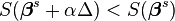for all sufficiently small . Thus, if divergence occurs, one solution is to employ a fraction, , of the increment vector, Δ in the updating formula

In other words, the increment vector is too long, but it points in "downhill", so going just a part of the way will decrease the objective function S. An optimal value for can be found by using a line search algorithm, that is, the magnitude of is determined by finding the value that minimizes S, usually using a direct search method in the interval .

In cases where the direction of the shift vector is such that the optimal fraction, , is close to zero, an alternative method for handling divergence is the use of the Levenberg–Marquardt algorithm, also known as the "trust region method".^[1] The normal equations are modified in such a way that the increment vector is rotated towards the direction of steepest descent,

where D is a positive diagonal matrix. Note that when D is the identity matrix and , then , therefore the direction of Δ approaches the direction of the negative gradient .

The so-called Marquardt parameter, , may also be optimized by a line search, but this is inefficient as the shift vector must be re-calculated every time is changed. A more efficient strategy is this. When divergence occurs increase the Marquardt parameter until there is a decrease in S. Then, retain the value from one iteration to the next, but decrease it if possible until a cut-off value is reached when the Marquardt parameter can be set to zero; the minimization of S then becomes a standard Gauss–Newton minimization.

The (non-negative) damping factor, , is adjusted at each iteration. If reduction of S is rapid, a smaller value can be used, bringing the algorithm closer to the Gauss–Newton algorithm, whereas if an iteration gives insufficient reduction in the residual, can be increased, giving a step closer to the gradient descent direction. Note that the gradient of S with respect to δ equals . Therefore, for large values of , the step will be taken approximately in the direction of the gradient. If either the length of the calculated step, δ, or the reduction of sum of squares from the latest parameter vector, β + δ, fall below predefined limits, iteration stops and the last parameter vector, β, is considered to be the solution.

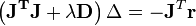
Levenberg's algorithm has the disadvantage that if the value of damping factor, , is large, inverting J^TJ + I is not used at all. Marquardt provided the insight that we can scale each component of the gradient according to the curvature so that there is larger movement along the directions where the gradient is smaller. This avoids slow convergence in the direction of small gradient. Therefore, Marquardt replaced the identity matrix, I, with the diagonal matrix consisting of the diagonal elements of J^TJ, resulting in the Levenberg–Marquardt algorithm:

Related algorithms

In a quasi-Newton method, such as that due to Davidon, Fletcher and Powell or Broyden–Fletcher–Goldfarb–Shanno (BFGS method) an estimate of the full Hessian,, is built up numerically using first derivatives only so that after n refinement cycles the method closely approximates to Newton's method in performance. Note that quasi-Newton methods can minimize general real-valued functions, whereas Gauss-Newton, Levenberg-Marquardt, etc. fits only to nonlinear least-squares problems.

Another method for solving minimization problems using only first derivatives is gradient descent. However, this method does not take into account the second derivatives even approximately. Consequently, it is highly inefficient for many functions, especially if the parameters have strong interactions.

非线性最优化（二）——高斯牛顿法和Levengerg-Marquardt迭代相关推荐

视觉SLAM十四讲学习笔记-第六讲-非线性优化的实践-高斯牛顿法和曲线拟合
专栏系列文章如下: 视觉SLAM十四讲学习笔记-第一讲_goldqiu的博客-CSDN博客视觉SLAM十四讲学习笔记-第二讲-初识SLAM_goldqiu的博客-CSDN博客视觉SLAM十四讲学习 ...
非线性最小二乘问题的高斯-牛顿算法
@非线性最小二乘问题的高斯-牛顿算法非线性最小二乘与高斯-牛顿算法开始做这个东西还是因为学校里的一次课程设计任务,找遍了全网好像也没有特别好用的,于是就自己写了一个.仅供参考. 首先,介绍下非线性 ...
高斯牛顿迭代法matlab代码,优化算法--牛顿迭代法
简书同步更新牛顿法给出了任意方程求根的数值解法,而最优化问题一般会转换为求函数之间在"赋范线性空间"的距离最小点,所以,利用牛顿法去求解任意目标函数的极值点是个不错的思路. 方程 ...
梯度下降、牛顿法、高斯牛顿L-M算法比较
本文梳理一下常见的几种优化算法:梯度下降法,牛顿法.高斯-牛顿法和L-M算法,优化算法根据阶次可以分为一阶方法(梯度下降法),和二阶方法(牛顿法等等),不同优化算法的收敛速度,鲁棒性都有所不同.一般来 ...
牛顿法和高斯牛顿法对比
文章目录一.非线性最小二乘一.牛顿法二.高斯牛顿法三.列文伯格-马夸尔特法(LM) 四.ceres求解优化问题一.非线性最小二乘考虑最小二乘函数F(x), 其等于: 通过求F(x)导数为零 ...
高斯牛顿(Gauss Newton)、列文伯格-马夸尔特(Levenberg-Marquardt)最优化算法与VSLAM
转载请说明出处:http://blog.csdn.net/zhubaohua_bupt/article/details/74973347 在VSLAM优化部分,我们多次谈到,构建一个关于待优化位姿的误 ...
视觉里程计 | 关于Stereo DSO中的高斯牛顿的一点注释
博主github:https://github.com/MichaelBeechan 博主CSDN:https://blog.csdn.net/u011344545 引子: 文章链接:https:// ...
线性和非线性最优化理论、方法及应用研究的发展状况.
关注. 最优化的研究包含理论.方法和应用.最优化理论主要研究问题解的最优性条件.灵敏度分析.解的存在性和一般复杂性等.而最优化方法研究包括构造新算法.证明解的收敛性.算法的比较和复杂性等.最优化的应用 ...
梯度下降法，牛顿法，高斯-牛顿迭代法，附代码实现
---------------------梯度下降法------------------- 梯度的一般解释: f(x)在x0的梯度:就是f(x)变化最快的方向.梯度下降法是一个最优化算法,通常也称为最 ...

非线性最优化（二）——高斯牛顿法和Levengerg-Marquardt迭代

非线性最优化（二）——高斯牛顿法和Levengerg-Marquardt迭代相关推荐

最新文章

热门文章