Time series analysis, discussed ARIMA, auto ARIMA, auto correlation (ACF), partial auto correlation (PACF), stationarity and differencing.

时间序列分析，讨论了ARIMA，自动ARIMA，自动相关(ACF)，部分自动相关(PACF)，平稳性和微分。

数据在哪里？ (Where is the data?)

Most financial time series examples use built-in data sets. Sometimes these data do not attend your needs and you face a roadblock if you don’t know how to get the exact data that you need.

大多数财务时间序列示例都使用内置数据集。 有时，这些数据无法满足您的需求，如果您不知道如何获取所需的确切数据，就会遇到障碍。

In this article I will demonstrate how to extract data directly from the internet. Some packages already did it, but if you need another related data, you will do it yourself. I will show you how to extract funds information directly from website. For the sake of demonstration, we have picked Brazilian funds that are located on CVM (Comissão de Valores Mobiliários) website, the governmental agency that regulates the financial sector in Brazil.

在本文中，我将演示如何直接从Internet提取数据。 一些软件包已经做到了，但是如果您需要其他相关数据，则可以自己完成。 我将向您展示如何直接从网站提取资金信息。 为了演示，我们选择了位于CVM(Comissãode ValoresMobiliários)网站上的巴西基金，该网站是监管巴西金融业的政府机构。

Probably every country has some similar institutions that store financial data and provide free access to the public, you can target them.

可能每个国家都有一些类似的机构来存储财务数据并向公众免费提供访问权限，您可以将它们作为目标。

从网站下载数据 (Downloading the data from website)

To download the data from a website we could use the function getURL from the RCurlpackage. This package could be downloaded from the CRAN just running the install.package(“RCurl”) command in the console.

要从网站下载数据，我们可以使用RCurlpackage中的getURL函数。 只需在控制台中运行install.package(“ RCurl”)命令，即可从CRAN下载此软件包。

downloading the data, url http://dados.cvm.gov.br/dados/FI/DOC/INF_DIARIO/DADOS/

下载数据，网址为http://dados.cvm.gov.br/dados/FI/DOC/INF_DIARIO/DADOS/

library(tidyverse) # a package to handling the messy data and organize itlibrary(RCurl) # The package to download a spreadsheet from a websitelibrary(forecast) # This package performs time-series applicationslibrary(PerformanceAnalytics) # A package for analyze financial/ time-series datalibrary(readr) # package for read_delim() function

#creating an object with the spreadsheet url url <- "http://dados.cvm.gov.br/dados/FI/DOC/INF_DIARIO/DADOS/inf_diario_fi_202006.csv"

#downloading the data and storing it in an R object text_data <- getURL(url, connecttimeout = 60)

#creating a data frame with the downloaded file. I use read_delim function to fit the delim pattern of the file. Take a look at it!df <- read_delim(text_data, delim = ";")

#The first six lines of the datahead(df)### A tibble: 6 x 8##   CNPJ_FUNDO DT_COMPTC  VL_TOTAL VL_QUOTA VL_PATRIM_LIQ CAPTC_DIA RESG_DIA##   <chr>      <date>        <dbl>    <dbl>         <dbl>     <dbl>    <dbl>## 1 00.017.02~ 2020-06-01 1123668.     27.5      1118314.         0        0## 2 00.017.02~ 2020-06-02 1123797.     27.5      1118380.         0        0## 3 00.017.02~ 2020-06-03 1123923.     27.5      1118445.         0        0## 4 00.017.02~ 2020-06-04 1124052.     27.5      1118508.         0        0## 5 00.017.02~ 2020-06-05 1123871.     27.5      1118574.         0        0## 6 00.017.02~ 2020-06-08 1123999.     27.5      1118639.         0        0## # ... with 1 more variable: NR_COTST <dbl>

处理凌乱 (Handling the messy)

This data set contains a lot of information about all the funds registered on the CVM. First of all, we must choose one of them to apply our time-series analysis.

该数据集包含有关在CVM上注册的所有资金的大量信息。 首先，我们必须选择其中之一来应用我们的时间序列分析。

There is a lot of funds for the Brazilian market. To count how much it is, we must run the following code:

巴西市场有很多资金。 要计算多少，我们必须运行以下代码：

#get the unique identification code for each fund x <- unique(df$CNPJ_FUNDO)

length(x) # Number of funds registered in Brazil.##[1] 17897

I selected the Alaska Black FICFI Em Ações — Bdr Nível I with identification code (CNPJ) 12.987.743/0001–86 to perform the analysis.

我选择了带有识别代码(CNPJ)12.987.743 / 0001–86的阿拉斯加黑FICFI EmAções-BdrNívelI来进行分析。

Before we start, we need more observations to do a good analysis. To take a wide time window, we need to download more data from the CVM website. It is possible to do this by adding other months to the data.

在开始之前，我们需要更多的观察资料才能进行良好的分析。 要花很长时间，我们需要从CVM网站下载更多数据。 可以通过在数据中添加其他月份来实现。

For this we must take some steps:

为此，我们必须采取一些步骤：

First, we must generate a sequence of paths to looping and downloading the data. With the command below, we will take data from January 2018 to July 2020.

首先，我们必须生成一系列循环和下载数据的路径。 使用以下命令，我们将获取2018年1月至2020年7月的数据。

# With this command we generate a list of urls for the years of 2020, 2019, and 2018 respectively.

 url20 <- c(paste0("http://dados.cvm.gov.br/dados/FI/DOC/INF_DIARIO/DADOS/inf_diario_fi_", 202001:202007, ".csv")) url19 <- c(paste0("http://dados.cvm.gov.br/dados/FI/DOC/INF_DIARIO/DADOS/inf_diario_fi_", 201901:201912, ".csv")) url18 <- c(paste0("http://dados.cvm.gov.br/dados/FI/DOC/INF_DIARIO/DADOS/inf_diario_fi_", 201801:201812, ".csv"))

After getting the paths, we have to looping trough this vector of paths and store the data into an object in the R environment. Remember that between all the 17897 funds, I select one of them, the Alaska Black FICFI Em Ações — Bdr Nível I

获取路径后，我们必须遍历该路径向量，并将数据存储到R环境中的对象中。 请记住，在所有的17897基金中，我选择其中一个，即阿拉斯加黑FICFI EmAções-BdrNívelI

# creating a data frame object to fill of funds information fundoscvm <- data.frame()

 # Loop through the urls to download the data and select the chosen investment fund. # This loop could take some time, depending on your internet connection. for(i in c(url18,url19,url20)){   csv_data <- getURL(i, connecttimeout = 60)   fundos <- read_delim(csv_data, delim = ";")

   fundoscvm <- rbind(fundoscvm, fundos)   rm(fundos) }

Now we could take a look at the new data frame called fundoscvm. This is a huge data set with 10056135 lines.

现在，我们可以看一下称为fundoscvm的新数据框。 这是一个包含10056135条线的庞大数据集。

Let’s now select our fund to be forecast.

现在让我们选择要预测的基金。

alaska <- fundoscvm%>%     filter(CNPJ_FUNDO == "12.987.743/0001-86") # filtering for the `Alaska Black FICFI Em Ações - Bdr Nível I` investment fund.# The first six observations of the time-series head(alaska)## # A tibble: 6 x 8 ##   CNPJ_FUNDO DT_COMPTC  VL_TOTAL VL_QUOTA VL_PATRIM_LIQ CAPTC_DIA RESG_DIA ##   <chr>      <date>        <dbl>    <dbl>         <dbl>     <dbl>    <dbl> ## 1 12.987.74~ 2018-01-02   6.61e8     2.78    630817312.  1757349. 1235409. ## 2 12.987.74~ 2018-01-03   6.35e8     2.78    634300534.  5176109. 1066853. ## 3 12.987.74~ 2018-01-04   6.50e8     2.82    646573910.  3195796.  594827. ## 4 12.987.74~ 2018-01-05   6.50e8     2.81    647153217.  2768709.  236955. ## 5 12.987.74~ 2018-01-08   6.51e8     2.81    649795025.  2939978.  342208. ## 6 12.987.74~ 2018-01-09   6.37e8     2.78    646449045.  4474763.   27368. ## # ... with 1 more variable: NR_COTST <dbl># The las six observations... tail(alaska)## # A tibble: 6 x 8 ##   CNPJ_FUNDO DT_COMPTC  VL_TOTAL VL_QUOTA VL_PATRIM_LIQ CAPTC_DIA RESG_DIA ##   <chr>      <date>        <dbl>    <dbl>         <dbl>     <dbl>    <dbl> ## 1 12.987.74~ 2020-07-24   1.89e9     2.46   1937895754.   969254.  786246. ## 2 12.987.74~ 2020-07-27   1.91e9     2.48   1902905141.  3124922. 2723497. ## 3 12.987.74~ 2020-07-28   1.94e9     2.53   1939132315.   458889.       0  ## 4 12.987.74~ 2020-07-29   1.98e9     2.57   1971329582.  1602226.  998794. ## 5 12.987.74~ 2020-07-30   2.02e9     2.62   2016044671.  2494009. 2134989. ## 6 12.987.74~ 2020-07-31   1.90e9     2.47   1899346032.   806694. 1200673. ## # ... with 1 more variable: NR_COTST <dbl>

The CVM website presents a lot of information about the selected fund. We are interested only in the fund share value. This information is in the VL_QUOTAvariable. With the share value, we could calculate several financial indicators and perform its forecasting.

CVM网站提供了许多有关所选基金的信息。 我们只对基金份额价值感兴趣。 此信息在VL_QUOTA变量中。 利用股票价值，我们可以计算几个财务指标并进行预测。

The data dimension is 649, 8. The period range is:

数据维度为649、8。周期范围为：

# period range: range(alaska$DT_COMPTC)## [1] "2018-01-02" "2020-07-31"

Let´s see the fund share price.

让我们看看基金的股价。

ggplot(alaska, aes( DT_COMPTC, VL_QUOTA))+ geom_line()+   scale_x_date(date_breaks = "3 month") +   theme(axis.text.x=element_text(angle=60, hjust=1))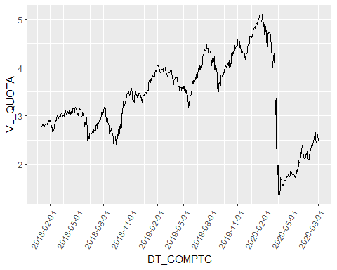

COVID-19 brings a lot of trouble, doesn’t it?

COVID-19带来很多麻烦，不是吗？

A financial raw series probably contains some problems in the form of patterns that repeat overtime or according to the economic cycle.

原始金融系列可能包含一些问题，这些问题的形式是重复加班或根据经济周期。

A daily financial time series commonly has a 5-period seasonality because of the trading days of the week. Some should account for holidays and other days that the financial market does not work. I will omit these cases to simplify the analysis.

由于一周中的交易日，每日财务时间序列通常具有5个周期的季节性。 有些人应该考虑假期以及金融市场无法正常运作的其他日子。 我将省略这些案例以简化分析。

We can observe in the that the series seems to go upward during a period and down after that. This is a good example of a trend pattern observed in the data.

我们可以观察到，该系列似乎在一段时间内上升，然后下降。 这是在数据中观察到的趋势模式的一个很好的例子。

It is interesting to decompose the series to see “inside” the series and separate each of the effects, to capture the deterministic (trend and seasonality) and the random (remainder) parts of the financial time-series.

分解序列以查看序列“内部”并分离每种影响，以捕获金融时间序列的确定性(趋势和季节性)和随机性(剩余)部分，这很有趣。

分解系列 (Decomposing the series)

A time-series can be decomposed into three components: trend, seasonal, and the remainder (random).

时间序列可以分解为三个部分：趋势，季节和其余部分(随机)。

There are two ways that we could do this: The additive form and the multiplicative form.

我们可以通过两种方式执行此操作：加法形式和乘法形式。

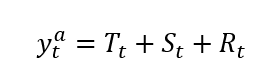
Let y_t be our time-series, T_t represents the trend, S_t is the seasonal component, and R_t is the remainder, or random component.In the additive form, we suppose that the data structure is the sum of its components:

假设y_t是我们的时间序列，T_t代表趋势，S_t是季节性成分，R_t是余数或随机成分。以加法形式，我们假设数据结构是其成分之和：

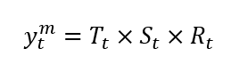
In the multiplicative form, we suppose that the data structure is a product of its components:

以乘法形式，我们假设数据结构是其组成部分的乘积：

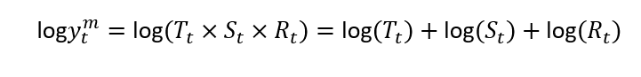
These structures are related. The log of a multiplicative structure is an additive structure of the (log) components:

这些结构是相关的。 乘法结构的对数是(log)组件的加法结构：

Setting a seasonal component of frequency 5, we could account for the weekday effect of the fund returns. We use five because there is no data for the weekends. You also should account for holidays, but since it vary according to the country on analysis, I ignore this effect.

设置频率为5的季节性成分，我们可以考虑基金收益的平日影响。 我们使用五个，因为没有周末的数据。 您还应该考虑假期，但是由于分析时会因国家/地区而异，因此我忽略了这种影响。

library(stats) # a package to perform and manipulate time-series objects library(lubridate) # a package to work with date objects library(TSstudio) # A package to handle time-series data

 # getting the starting point of the time-series data start_date <- min(alaska$DT_COMPTC)

 # The R program does not know that we are working on time-series. So we must tell the software that our data is a time-series. We do this using the ts() function

 ## In the ts() function we insert first the vector that has to be handle as a time-series. Second, we tell what is the starting point of the time series. Third, we have to set the frequency of the time-series. In our case, it is 5. share_value <- ts(alaska$VL_QUOTA, start =start_date, frequency = 5)

 # the function decompose() performs the decomposition of the series. The default option is the additive form. dec_sv <- decompose(share_value)

 # Take a look! plot(dec_sv)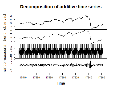

Decomposition of additive time series.

分解附加时间序列。

The above figure shows the complete series observed, and its three components trend, seasonal, and random, decomposed in the additive form.

上图显示了观察到的完整序列，其三个成分趋势(季节性和随机)以加法形式分解。

The below figure shows the complete series observed, and its three components trend, seasonal, and random, decomposed in the multiplicative form.

下图显示了观察到的完整序列，其三个分量趋势(季节性和随机)以乘法形式分解。

The two forms are very related. The seasonal components change slightly.

两种形式非常相关。 季节成分略有变化。

dec2_sv <- decompose(share_value, type = "multiplicative")

 plot(dec2_sv)

In a time-series application, we are interested in the return of the fund. Another information from the related data set is useless to us.

在时间序列应用程序中，我们对基金的回报感兴趣。 来自相关数据集的另一个信息对我们没有用。

The daily return (Rt) of a fund is obtained from the (log) first difference of the share value. In your data, his variables call VL_QUOTA. The logs are important because give to us a proxy of daily returns in percentage.

基金的日收益率(R t )是从股票价值的(对数)第一差得出的。 在您的数据中，他的变量称为VL_QUOTA。 日志很重要，因为可以按百分比为我们提供每日收益的代理。

The algorithm for this is:

其算法为：

R1 <- log(alaska$VL_QUOTA)%>% # generate the log of the series   diff() # take the first difference

 plot.ts(R1) # function to plot a time-series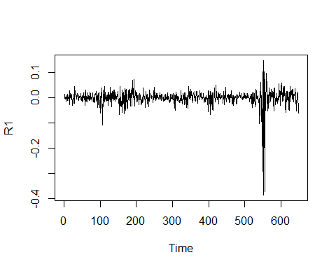

The return (log-first difference) series takes the role of the remainder in the decomposition did before.

返回(对数优先差)序列在之前的分解过程中承担其余部分的作用。

The random component of the decomposed data is seasonally free. We could do this by hand taking a 5-period difference:

分解后的数据的随机成分在季节性上不受限制。 我们可以手动进行5个周期的区别：

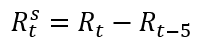
R5 <- R1 %>% diff(lag = 5) plot.ts(R5)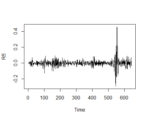

The two graphs are similar. But the second does not have a possible seasonal effect.

这两个图是相似的。 但是第二个并没有可能的季节性影响。

We can plot a graph to identify visually the seasonality of the series using the ggsubseriesplot function of the forecastpackage.

我们可以绘制图表以使用Forecastpackage的ggsubseriesplot函数直观地识别系列的季节性。

ggsubseriesplot(share_value)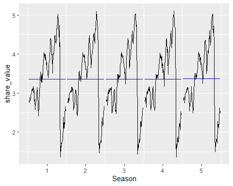

Oh, it seems that our hypothesis for seasonal data was wrong! There is no visually pattern of seasonality in this time-series.

哦，看来我们对季节性数据的假设是错误的！ 在此时间序列中，没有视觉上的季节性模式。

预测 (The Forecasting)

Before forecasting, we have to verify if the data are random or auto-correlated. To verify autocorrelation in the data we can first use the autocorrelation function (ACF) and the partial autocorrelation function (PACF).

进行预测之前，我们必须验证数据是随机的还是自动相关的。 为了验证数据中的自相关，我们可以首先使用自相关函数(ACF)和部分自相关函数(PACF)。

自相关函数和部分自相关函数 (Autocorrelation Function and Partial Autocorrelation Function)

If we use the raw data, the autocorrelation is evident. The blue line indicates that the significance limit of the lag’s autocorrelation. In the below ACF figure, the black vertical line overtaking the horizontal blue line means that the autocorrelation is significant at a 5% confidence level. The sequence of upward lines indicate positive autocorrelation for the tested series.

如果我们使用原始数据，则自相关是明显的。 蓝线表示滞后自相关的显着性极限。 在下面的ACF图中，黑色的垂直线超过水平的蓝线表示自相关在5％的置信度下很重要。 向上的线序列表示测试序列的正自相关。

To know the order of the autocorrelation, we have to take a look on the Partial Autocorrelation Function (PACF).

要知道自相关的顺序，我们必须看一下部分自相关函数(PACF)。

library(TSstudio)

 R <- alaska$VL_QUOTA #extract the fund share value from the data Racf <- acf(R, lag.max = 12) # compute the ACF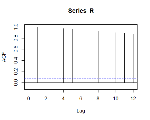

Autocorrelation Function for the fund share value.

基金份额价值的自相关函数。

Rpacf <- pacf(R, lag.max = 12) # compute the PACF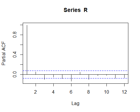

The Partial Autocorrelation Function confirms the autocorrelation in the data for lags 1, 6,and 8.

部分自相关函数可确认数据中的自相关，分别用于滞后1、6和8。

At the most of time, in a financial analysis we are interested on the return of the fund share. To work with it, one can perform the forecasting analysis to the return rather than use the fund share price. I add to you that this procedure is a good way to handle with the non-stationarity of the fund share price.

在大多数时候，在财务分析中，我们对基金份额的回报很感兴趣。 要使用它，人们可以对收益进行预测分析，而不必使用基金股票的价格。 我要补充一点，此程序是处理基金股票价格不稳定的好方法。

So, we could perform the (partial) autocorrelation function of the return:

因此，我们可以执行返回的(部分)自相关函数：

library(TSstudio)

 Racf <- acf(R1, lag.max = 12) # compute the ACF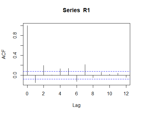

ACF for the fund share (log) Return.

基金份额(日志)收益的ACF。

Racf <- acf(R5, lag.max = 12) # compute the ACF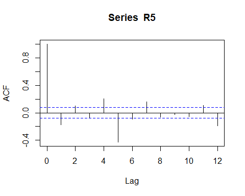

Above ACF figure suggests a negative autocorrelation pattern, but is impossible identify visually the exactly order, or if exists a additional moving average component in the data.

ACF上方的数字表示自相关模式为负，但无法从视觉上确定确切的顺序，或者如果数据中存在其他移动平均成分，则无法确定。

Rpacf <- pacf(R1, lag.max = 12) # compute the PACF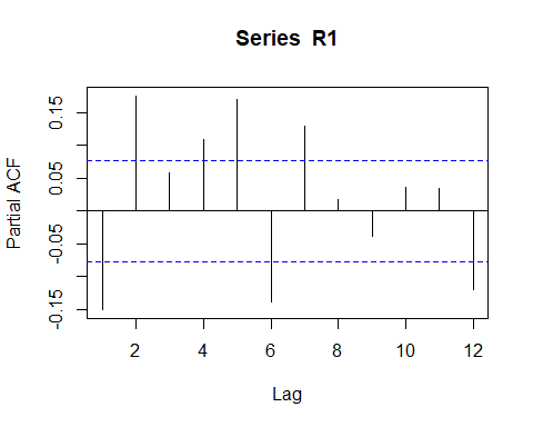

PACF for the fund share (log) Return.

基金份额的PACF(日志)回报。

Rpacf <- pacf(R5, lag.max = 12) # compute the PACF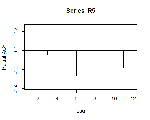

autocorrelation function of the Return does not help us so much. Only that we can set is that exist a negative autucorrelation pattern.

Return的自相关函数对我们没有太大帮助。 我们唯一可以设置的是存在负的自相关模式。

One way to identify what is the type of components to be used ( autocorrelation or moving average). We could perform various models specifications and choose the model with better AIC or BIC criteria.

一种识别要使用的组件类型(自相关或移动平均值)的方法。 我们可以执行各种模型规范，并选择具有更好AIC或BIC标准的模型。

使用ARIMA模型进行预测 (Forecasting with ARIMA models)

One good option to perform a forecasting model is to use the family of ARIMA models. For who that is not familiar with theoretical stuff about ARIMA models or even Autocorrelation Functions, I suggest the Brooks books, “Introductory Econometrics for Finance”.

执行预测模型的一个不错的选择是使用ARIMA模型系列。 对于那些不熟悉ARIMA模型甚至自相关函数的理论知识的人，我建议使用Brooks的著作“金融计量经济学入门”。

To model an ARIMA(p,d,q) specification we must to know the order of the autocorrelation component (p), the order of integration (d), and the order of the moving average process (q).

要对ARIMA(p，d，q)规范建模，我们必须知道自相关分量的阶数(p)，积分阶数(d)和移动平均过程阶数(q)。

OK, but, how to do that?

好的，但是，该怎么做呢？

The first strategy is to look to the autocorrelation function and the partial autocorrelation function. since we cant state just one pattern based in what we saw in the graphs, we have to test some model specifications and choose one that have the better AIC or BIC criteria.

第一种策略是考虑自相关函数和部分自相关函数。 由于我们不能根据图中看到的仅陈述一种模式，因此我们必须测试一些模型规格并选择一种具有更好的AIC或BIC标准的规格。

We already know that the Returns are stationary, so we do not have to verify stationary conditions (You do it if you don’t trust me :).

我们已经知道退货是固定的，因此我们不必验证固定的条件(如果您不信任我，请这样做：)。

# The ARIMA regression arR <- Arima(R5, order = c(1,0,1)) # the auto.arima() function automatically choose the optimal lags to AR and MA components and perform tests of stationarity and seasonality

 summary(arR) # now we can see the significant lags## Series: R5  ## ARIMA(1,0,1) with non-zero mean  ##  ## Coefficients: ##           ar1     ma1    mean ##       -0.8039  0.6604  0.0000 ## s.e.   0.0534  0.0636  0.0016 ##  ## sigma^2 estimated as 0.001971:  log likelihood=1091.75 ## AIC=-2175.49   AICc=-2175.43   BIC=-2157.63 ##  ## Training set error measures: ##                        ME       RMSE        MAE      MPE     MAPE      MASE ## Training set 9.087081e-07 0.04429384 0.02592896 97.49316 192.4589 0.6722356 ##                     ACF1 ## Training set 0.005566003

If you want a fast analysis than perform several models and compare the AIC criteria, you could use the auto.arima() functions that automatically choose the orders of autocorrelation, integration and also test for season components in the data.

如果要进行快速分析而不是执行多个模型并比较AIC标准，则可以使用auto.arima()函数自动选择自相关，积分的顺序，并测试数据中的季节成分。

I use it to know that the ARIMA(1,0,1) is the best fit for my data!!

我用它知道ARIMA(1,0,1)最适合我的数据！！

It is interesting to check the residuals to verify if the model accounts for all non random component of the data. We could do that with the checkresiduals function of the forecastpackage.

检查残差以验证模型是否考虑了数据的所有非随机成分是很有趣的。 我们可以使用Forecastpackage的checkresiduals函数来做到这一点。

checkresiduals(arR)# checking the residuals

 ##  ##  Ljung-Box test ##  ## data:  Residuals from ARIMA(1,0,1) with non-zero mean ## Q* = 186.44, df = 7, p-value < 2.2e-16 ##  ## Model df: 3.   Total lags used: 10

Look to the residuals ACF. The model seem to not account for all non-random components, probably by an conditional heteroskedasticity. Since it is not the focus of the post, you could Google for Arch-Garch family models

查看残差ACF。 该模型似乎没有考虑到所有非随机成分，可能是由于条件异方差性造成的。 由于不是本文的重点，因此您可以将Google用于Arch-Garch系列模型

现在，预测！ (Now, the forecasting!)

Forecasting can easily be performed with a single function forecast. You should only insert the model object given by the auto.arima() function and the periods forward to be foreseen.

可以使用单个功能预测轻松进行预测。 您应该只插入由auto.arima()函数给定的模型对象以及可以预见的周期。

farR <-forecast(arR, 15)

 ## Fancy way to see the forecasting plot

 plot_forecast(farR)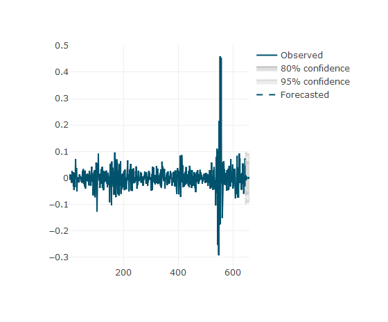

The function plot_forecast of the TSstudio package is a nice way to see the plot forecasting. If you pass the mouse cursor over the plot you cold see the cartesian position of the fund share.

TSstudio软件包的plot_forecast函数是查看情节预测的好方法。 如果将鼠标指针移到该图上，您会冷眼看到基金份额的笛卡尔位置。

Now you can go to predict everything that you want. Good luck!

现在，您可以预测所需的一切。 祝好运！