hotelling变换

背景 (Background)

One of the most common challenges encountered in the modeling of spectroscopic data is to select a subset of variables (i.e. wavelengths) out of a large number of variables associated with the response variable. It is common for spectroscopic data to have a large number of variables relative to the number of observations. In such a situation, the selection of a smaller number of variables is crucial especially if we want to speed up the computation time and gain in the model’s stability and interpretability. Typically, variable selection methods are classified into two groups:

在光谱数据的建模中遇到的最常见的挑战Òne为选择的变量的子集(即，波长)了大量的与该响应相关联的变量的变量。光谱数据相对于观测数量通常具有大量变量。在这种情况下，选择较小数量的变量至关重要，尤其是在我们希望加快计算时间并提高模型稳定性和可解释性的情况下。通常，变量选择方法分为两类：

• Filter-based methods: the most relevant variables are selected as a preprocessing step independently of the prediction model.• Wrapper-based methods: use the supervised learning approach.

•基于过滤器的方法：与预测模型无关，选择最相关的变量作为预处理步骤。•基于包装器的方法：使用监督学习方法。

Hence, any PLS-based variable selection is a wrapper method. Wrapper methods need a selection criterion that relies solely on the characteristics of the data at hand.

因此，任何基于PLS的变量选择都是包装器方法。包装方法需要一个选择标准，该选择标准仅依赖于手头数据的特征。

方法 (Method)

Let us consider a regression problem for which the relation between the response variable y (n × 1) and the predictor matrix X (n × p) is assumed to be explained by the linear model y = β X, where β (p × 1) is the regression coefficients. Our dataset is comprised of n = 466 observations from various plant materials, and y corresponds to the concentration of calcium (Ca) for each plant. The matrix X is our measured LIBS spectra that includes p = 7151 wavelength variables. Our objective is therefore to find some columns subsets of X with satisfactorily predictive power for the Ca content.

让我们考虑假定的量，响应变量Y(N×1)和预测器矩阵X(N×P)之间的关系由线性模型Y =βX，其中β(P×1说明一个回归问题)是回归系数。我们的数据集由来自各种植物材料的n = 466个观测值组成，并且y对应于每种植物的钙(Ca)浓度。矩阵X是我们测得的LIBS光谱，其中包括p = 7151个波长变量。因此，我们的目标是找到一些X的子集，这些子集对于Ca含量具有令人满意的预测能力。

ROBPCA建模 (ROBPCA modeling)

Let’s first perform robust principal components analysis (ROBPCA) to help visualize our data and detect whether there is an unusual structure or pattern. The obtained scores are illustrated by the scatterplot below in which the ellipses represent the 95% and 99% confidence interval from the Hotelling’s T². Most observations are below the 95% confidence level, albeit some observations seem to cluster on the top-right corner of the scores scatterplot.

让我们首先执行健壮的主成分分析( ROBPCA )，以帮助可视化我们的数据并检测是否存在异常的结构或模式。所获得的分数由下面的散点图说明，其中椭圆表示距Hotelling T 2的95％和99％置信区间。尽管有些观察似乎聚集在分数散点图的右上角，但大多数观察都低于95％的置信度。

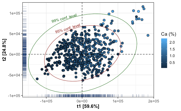
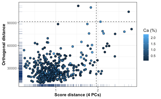
However, when looking more closely, for instance using the outlier map, we can see that ultimately there are only three observations that seem to pose a problem. We have two observations flagged as orthogonal outliers and only one as a bad leverage point. Some observations are flagged as good leverage points, whilst most are regular observations.

但是，当更仔细地观察时(例如，使用离群值地图)，我们可以看到最终只有三个观测值似乎构成问题。我们有两个观测值标记为正交离群值，只有一个观测值标记为不良杠杆点。一些观察值被标记为良好的杠杆点，而大多数是常规观察值。

PLS建模 (PLS modeling)

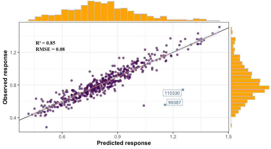
It is worth mentioning that in our regression problem, ordinary least square (OLS) fitting is no option since n ≪ p. PLS resolves this by searching for a small set of the so-called latent variables (LVs), that performs a simultaneous decomposition of X and y with the constraint that these components explain as much as possible of the covariance between X and y. The figures below are the results obtained from the PLS model. We obtained an R² of 0.85 with an RMSE and MAE of 0.08 and 0.06, respectively, which correspond to a mean absolute percentage error (MAPE) of approximately 7%.

值得一提的是，在我们的回归问题，普通最小二乘法(OLS)拟合是由于N“P别无选择。 PLS通过搜索一小组所谓的潜在变量(LVs)来解决此问题，该变量在约束X和y尽可能解释X和y之间的协方差的约束下执行X和y的同时分解。下图是从PLS模型获得的结果。我们获得的R²为0.85，RMSE和MAE分别为0.08和0.06，这对应于大约7％的平均绝对百分比误差(MAPE)。

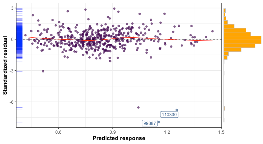
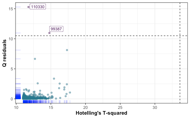
Observed vs. predicted plot (full dataset).

Similarly to the ROBPCA outlier map, the PLS residual plot has flagged three observations that exhibit high standardized residual value. Another way to check for outliers is to calculate Q-residuals and Hotelling’s T² from the PLS model, then define a criterion for which an observation is considered as an outlier or not. High Q-residual value corresponds to an observation which is not well explained by the model, while high Hotelling’s T² value expresses an observation that is far from the center of regular observations (i.e, score = 0). The results are plotted below.

与ROBPCA离群图相似，PLS残差图标记了三个观测值，这些观测值表现出较高的标准残差值。检查异常值的另一种方法是从PLS模型计算Q残差和Hotelling的T²，然后定义一个标准，对于该标准，观察值是否视为异常值。高Q残差值对应于模型无法很好解释的观测值，而高Hotelling的T²值表示远离常规观测值中心的观测值(即，得分= 0)。结果绘制在下面。

Q residuals vs. Hotelling’s T² plot (full dataset).

基于Hotelling-T²的变量选择 (Hotelling-T² based variable selection)

Let’s now perform variable selection from our PLS model, which is carried out by computing the T² statistic (for more details see Mehmood, 2016),

现在，让我们从我们的PLS模型中执行变量选择，该模型是通过计算T²统计信息来实现的(有关更多详细信息，请参阅Mehmood，2016 )，

where W is the loading weight matrix and C is the covariance matrix. Thus, a variable is selected based on the following criteria,

其中W是装载权重矩阵， C是协方差矩阵。因此，根据以下条件选择变量：

where A is number of LVs from our PLS model, and 1-

hotelling变换_基于Hotelling-T²的偏最小二乘（PLS）中的变量选择相关推荐

基于Python（sklearn）计算PLS中的VIP值
基于Python(sklearn)计算PLS中的VIP值 sklearn中PLS回归模型并没有计算VIP值的方法,但VIP又是很重要的筛选变量方法.下附代码思路与完整代码,若有错误,万望指正. 1.首 ...
指纹图谱相似度评价软件_基于指纹图谱和网络药理学对当归四逆汤中桂枝的Qmarker预测分析...
摘要:目的基于指纹图谱和网络药理学分析预测当归四逆汤(DSD)中桂枝的质量标志物(Q-marker).方法建立桂枝水煎液和DSD的指纹图谱,利用中药色谱指纹图谱相似度评价系统软件(2012年 ...
python偏最小二乘法回归分析_【数学建模】偏最小二乘回归分析（PLSR）
PLSR的基本原理与推导,我在这篇博客中有讲过. 0. 偏最小二乘回归集成了多元线性回归.主成分分析和典型相关分析的优点,在建模中是一个更好的选择,并且MATLAB提供了完整的实现,应用时主要的问题是 ...
多元线性回归算法: 线性回归Linear Regression、岭回归Ridge regression、Lasso回归、主成分回归PCR、偏最小二乘PLS
0. 问题描述输入数据:X=(x1,x2,....,xm)\mathbf{X} = (x_1, x_2,...., x_m)X=(x1,x2,....,xm), 相应标签 Y=(y1,y2,. ...
偏最小二乘(PLS)原理分析Python实现
目录 1 偏最小二乘的意义 2 PLS实现步骤 3 弄懂PLS要回答的问题 4 PLS的原理分析 4.1 自变量和因变量的主成分求解原理 4.1.1 确定目标函数 4.1 ...
R实战 | OPLS-DA（正交偏最小二乘判别分析)筛选差异变量(VIP)及其可视化
主成分分析(PCA)是一种无监督降维方法,能够有效对高维数据进行处理.但PCA对相关性较小的变量不敏感,而PLS-DA(偏最小二乘判别分析)能够有效解决这个问题.而OPLS-DA(正交偏最小二乘判别分 ...
r语言pls分析_R语言中的偏最小二乘PLS回归算法
偏最小二乘回归: 我将围绕结构方程建模(SEM)技术进行一些咨询,以解决独特的业务问题.我们试图识别客户对各种产品的偏好,传统的回归是不够的,因为数据集的高度分量以及变量的多重共线性.PLS是处理这些 ...
图像mnf正变换_基于MNF 变换的多元变化检测变化信息的集中
展开全部 (一)基于MNF变换的变化信息集中的基本流程 MNF变换是一种多元62616964757a686964616fe58685e5aeb931333433616234线性统计变换方法,是针对一组 ...
three.js加载3d模型_基于WebGL的3D技术在网页中的运用 ThingJS 前端开发
Three.js.ThingJS这些引擎库可以加载3D制作软件的模型,大幅度提高了制作效率,改变WebGL开发困难的局面,让Web开发者享受便捷的3D开发服务.三者的难度对比如下: ThingJS(框 ...

hotelling变换_基于Hotelling-T²的偏最小二乘（PLS）中的变量选择