In this post, I will compare the output of frequentist and Bayesian statistics, and explain how these two approaches can be complementary, in particular for unclear results resulting from a frequentist approach.

在这篇文章中，我将比较常客和贝叶斯统计的输出，并解释这两种方法如何互补，特别是对于常客方法产生的不确定结果。

For a first proof of concept, I will use the famous Titanic data set, that every first Kaggle user is exposed to upon registration. These statistics can be of course applied on any other data set. I selected the Titanic data set because it has a large range of variables, and readers might already know the data.

作为第一个概念验证，我将使用著名的Titanic数据集，每个第一个Kaggle用户在注册时都会接触到它。 这些统计信息当然可以应用于任何其他数据集。 我选择“泰坦尼克号”数据集是因为它具有广泛的变量范围，并且读者可能已经知道这些数据。

For the ones not familiar with this data set, it offers a range of variables that can be used to predict the likelihood of having survived the accident that sunk the boat back then. You will find all kind of approaches online to analyze this data set, as well as machine learning techniques to predict survival.

对于不熟悉此数据集的人，它提供了一系列变量，可用于预测当时沉没在事故中幸存下来的可能性。 您将在线找到用于分析该数据集的各种方法，以及用于预测生存率的机器学习技术。

I downloaded it from some source on the net, and you can find the exact data set I used here.

我是从网上的一些来源下载的，您可以在这里找到我使用的确切数据集。

FYI, the variables are listed below:

仅供参考，以下列出了变量：

[print(i) for i in df.columns]PassengerIdSurvivedPclassNameSexAgeSibSpParchTicketFareCabinEmbarked

缺乏证据 (Absence of Evidence)

If you do the analysis yourself, you will find out that some variables are pretty good at predicting survival. For the sake of argumentation, and because I think it offers a nice explanatory power, let’s look at the variable age:

如果您自己进行分析，您会发现某些变量非常擅长预测存活率。 为了论证，并且因为我认为它提供了很好的解释能力，让我们看一下可变年龄：

df.Age.plot(kind='hist')

Since we want to investigate the effect of age on survival, let’s split that accordingly:

由于我们想研究年龄对生存的影响，因此我们将其相应地拆分：

(df.groupby('Survived').apply(lambda d: pd.Series({    "std": d.Age.std(),    "sem": d.Age.std() /  d.Age.count(),    "avg": d.Age.mean()})).plot(kind='barh',        y = "avg",        legend = False,        title = "Mean Age per Surival Class +/- std",        xerr = "std"      ));

From a simple bar plot, there does not seem to be a crazy difference in the age of passengers that survived and did not survived the accident. Looking at the error bars, we might think that these distributions are not significantly different.

从简单的条形图来看，幸存和未幸免于事故的乘客年龄似乎没有疯狂的差异。 查看误差线，我们可能会认为这些分布没有显着差异。

Let’s test that statistically.

让我们进行统计测试。

For the demonstration of Bayesian statistics, I will be using the open source software JASP, which offers a user-friendly interface. There are many other packages out there that would allow you to run Bayesian stats from code. Since the readers might not be well versed in code, I use this software to show how to run basic Bayesian testing.

为了演示贝叶斯统计，我将使用开源软件JASP ，它提供了用户友好的界面。 还有许多其他软件包，可让您从代码中运行贝叶斯统计信息。 由于读者可能不精通代码，因此我使用此软件来演示如何运行基本的贝叶斯测试。

Let’s first load the Titanic data set in JASP:

让我们首先在JASP中加载Titanic数据集：

Above you can see that JASP automatically reorganizes the data in columns in a nice readable way.

在上面可以看到，JASP以一种很好的可读方式自动重新组织了列中的数据。

JASP allows you to perform basic statistical testing from both frequentist and Bayesian approaches. While I typically run my stats using SciPy, its kind of nice to have both approaches embedded in one software, so that you can compare the outputs easily.

JASP允许您从常客和贝叶斯方法中执行基本的统计测试。 虽然我通常使用SciPy运行统计数据，但将两种方法都嵌入一个软件中还是一件不错的事，这样您就可以轻松比较输出。

Let’s first start with the classic frequentist approach.

让我们首先从经典的常客方法开始。

Below, you see a screenshot of the JASP window that pops out when you want to do an independent sample t-test, which is what we should be doing if we want to test whether passengers that survived had a significantly different age than people that died due to the tragedy.

在下面，您会看到一个JASP窗口的屏幕截图，当您想进行独立的t检验时会弹出该窗口，如果要测试幸存的乘客的年龄是否与死者的年龄显着不同，我们应该这样做由于悲剧。

As you can see, there is a lot of options that one could change, such as the type of test (Student, Welch, Mann-Whitney if you want to do a non parametric test), whether you have a hypothesis for the testing (one or two sided test). Additionally, you can also obtain more descriptive statistics if you want to explore your dataset using JASP.

如您所见，有很多选项可以更改，例如测试的类型(如果要进行非参数测试，则为学生，韦尔奇，曼惠特尼)，是否对测试有假设(一面或两面测试)。 此外，如果要使用JASP浏览数据集，还可以获取更多的描述性统计信息。

I will just run a standard Student test, that is parametric testing. Before doing that, we should be checking whether assumptions for parametric testing are fulfilled by the distribution, but for the sake of demo, let’s assume they are.

我将运行一个标准的Student测试，即参数测试。 在此之前，我们应该检查分布是否满足参数测试的假设，但是为了演示起见，让我们假设它们是正确的。

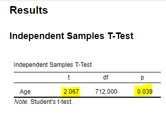
Quite surprisingly, the test shows a significant difference between the two distributions (t(712) = 2.067, P = 0.039), i.e., the observed difference in age is unlikely under the null hypothesis. The p-value really flirts with the typical 0.05 alpha level, suggesting that this effect is significant according to frequentist statistics, but not very convincing if I might add.

出乎意料的是，该测试显示了两种分布之间的显着差异(t(712)= 2.067，P = 0.039)，即，在原假设下，观察到的年龄差异不太可能。 p值确实与典型的0.05 alpha水平调情，这表明根据常客统计数据，这种影响是显着的，但是如果我添加的话，并不是很令人信服。

Before moving on, we should be looking at other measures than the p-value (effect size, see here, but since this post is about comparing frequentist and bayesian approach, I will just move on.

在继续之前，我们应该查看除p值(效果大小，请参见此处)之外的其他度量，但是由于本文是关于比较常客和贝叶斯方法的，因此我将继续。

Now let’s look at what a Bayesian Independent Sample t-test would show.

现在，让我们看一下贝叶斯独立样本t检验将显示什么。

The Bayesian test outputs a so-called Bayes Factor (BF), which is the relative predictive performance of the null hypothesis H0 versus the alternative hypothesis H1. See here for more information on Bayes Factor.

贝叶斯检验输出所谓的贝叶斯因子(BF)，它是零假设H0与替代假设H1的相对预测性能。 有关贝叶斯因子的更多信息，请参见此处 。

While I do not like the concept of arbitrary threshold, these ideas can be useful to draw meaningful conclusions about the data.

虽然我不喜欢任意阈值的概念，但是这些想法对于得出有意义的数据结论很有用。

In the frequentist world, the typical arbitrary threshold is 0.05, below which the effect is said to be significant.

在频繁的世界中，典型的任意阈值为0.05，低于该阈值则认为效果显着。

In the Bayesian world, and according to initial classifications by Jeffreys, the following nomenclature could be used:

在贝叶斯世界中，根据Jeffreys的初步分类，可以使用以下术语：

• BF < 1/3: evidence against the null hypothesis

  BF <1/3： 反对原假设的证据

• 1/3 < BF < 3 : Anecdotical evidence
  1/3 <BF <3：轶事证据

• BF > 3: Evidence for the null hypothesis

  BF> 3： 证据零假设

In our case, we select BF10, which represents the likelihood of the data under the 1 Hypothesis compared to the likelihood of the data under the null hypothesis (in math terms: p(data | H1) / p(data | H0)).

在我们的例子中，我们选择BF10，它表示1假设下的数据的可能性与零假设下的数据的可能性(以数学术语表示：p(data | H1)/ p(data | H0))。

Back to our test. We find interesting options in the main window, that would allow you to perform a one sided or two sided test (“Alt. Hypothesis”, indicate by “+” in JASP), as well as BF manipulations that allow you to calculate that ratio for each comparison, BF10 (hyp 1 vs hyp 0) and BF01 (reverse comparison).

回到我们的测试。 我们在主窗口中找到有趣的选项，使您可以执行单面或双面测试(“ Alt。Hypothesis”，在JASP中用“ +”表示)，以及BF操作，可以计算该比率对于每个比较，BF10(hyp 1 vs hyp 0)和BF01(反向比较)。

I suggest that you also explore the nice plots options that will allow you to visualize your prior and posterior distributions (that is for a separate post though…).

我建议您还探索漂亮的图选项，使您可以直观地看到之前和之后的分布(尽管这是一个单独的帖子……)。

Let’s run the test:

让我们运行测试：

In our case, we obtain a BF = 0.685, meaning that our data was 0.685 times more likely under H1 that under H0. According to initial classifications by Jeffreys, this speaks for a absence of evidence for H0, that is we cannot conclude that age does not affect the likelihood of survival in the Titanic accident. I insist here: since the BF is not below 1/3, we cannot claim that the have obtained evidence of the absence of effect of age on survival. In such situations, more data might be needed to observe how the BF might evolve with more accumulating data.

在我们的情况下，我们获得BF = 0.685，这意味着我们的数据在H1下的可能性是H0下的0.685倍。 根据杰弗里斯(Jeffreys)的初步分类，这表示没有H0的证据，也就是说，我们不能得出结论，年龄不会影响泰坦尼克号事故中幸存的可能性。 我在这里坚持认为：由于BF不低于​​1/3 ，我们不能断言该证据已获得年龄对生存没有影响的证据。 在这种情况下，可能需要更多的数据才能观察到BF随着更多的累积数据如何发展。

I like to think of Bayes Factor in the following terms: “How much should I change my belief that age has an impact on the survival likelihood of the titanic disaster?”. The answer is the Bayes Factor. Depending on your prior belief (that would be the so-called prior, that you can adapt based on what you already know from the data), the BF will be then different, depending on the strength of the effect.

我喜欢用以下术语来思考贝叶斯因素：“我应该改变多少看法，即年龄对泰坦尼克号灾难的生存可能性有影响？”。 答案是贝叶斯因子。 根据您之前的信仰(这将是前所谓的，你可以根据你已经从数据知道适应)，高炉将是那么的不同，这取决于效果的强度。

Here, it seems that I should not change my belief by much.

在这里，看来我不应该改变太多信念。

As you can see, while the frequentist approach would conclude of an effect of age, the bayesian one would say the more data is required before concluding. In such cases, the best would be to collect more data to get evidence of effect, or prove an evidence of absence of effect.

如您所见，尽管常人主义方法会得出年龄影响的结论，但贝叶斯主义者会说，得出结论之前需要更多数据。 在这种情况下，最好的方法是收集更多数据以获取效果的证据 ，或证明不存在效果的证据 。

效力证据 (Evidence of Effect)

Let’s now use another famous dataset, the boston housing dataset, to explore another situation. You can find this dataset on the repo given at the beginning of the post.

现在，让我们使用另一个著名的数据集，波士顿房屋数据集，来探索另一种情况。 您可以在帖子开头给出的回购中找到此数据集。

Below I am plotting the price of the houses (which you are supposed to predict in the initial competition), per location on or away from the Charles River.

在下面，我绘制了查尔斯河上或远离查尔斯河的每个位置的房屋价格(您应该在最初的竞争中进行预测)。

(df_housing.groupby('chas').apply(lambda d: pd.Series({    "std": d.medv.std(),    "sem": d.medv.std() /  d.medv.count(),    "avg": d.medv.mean()})).plot(kind='barh',        y = "avg",        legend = False,        title = "Mean price per river location +/- std",        xerr = "std"      ));

As we can see, the prices are higher for True values (close to the Charles River) than for False values. Now, let’s explore this observation statistically.

如我们所见，True值(靠近查尔斯河)的价格比False值高。 现在，让我们从统计学角度探索这一观察。

I won’t be showing the screenshots of the JASP results here, but only the results.

我不会在这里显示JASP结果的屏幕截图，而只会显示结果。

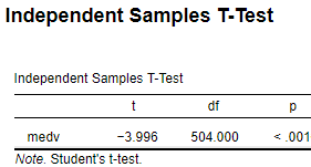
A frequentist independent sample t-test shows a highly significant difference between the two distributions (t(504) = -3.996, p < 0.001), i.e., the observed difference in housing price is significant between accomodations located on and away from the Charles River.

独立的t检验样本表明，两种分布之间的差异非常显着(t( 504 )= -3.996， p <0.001)，即，在查尔斯河上和远离查尔斯河的住宿中，观察到的房价差异均很大。

Let’s see what we obtain with a bayesian test.

让我们看看通过贝叶斯测试得到的结果。

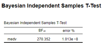
The bayesian approach confirms that observations with a very high BF value, suggesting that the data is 270 times more likely under the H1 hypothesis, than under the H0.

贝叶斯方法证实了BF值非常高的观测结果，这表明在H1假设下，数据的可能性是在H0下的270倍。

Now, we have the last case to explore: where bayesian statistics would allow us to conclude on the absence of an effect.

现在，我们要探讨的最后一个案例是：贝叶斯统计量可以使我们在没有影响的情况下得出结论。

缺席证据 (Evidence of Absence)

So far, so good. In the previous example, we saw that both approaches made sense and concurred when the effect is high. Now let’s look at another variable where we might be able to use the power of the bayesian approach a bit more clearly.

到目前为止，一切都很好。 在前面的示例中，我们看到两种方法都是有意义的，并且在效果很高时会同时存在。 现在，让我们看一下另一个变量，在该变量中我们可以更加清楚地使用贝叶斯方法的功能。

Instead of looking at a variable that is likely to show a difference in price, let’s look at another one: the “zn” variable, i.e., the proportion of residential land zoned for lots over 25,000 sq.ft.

让我们看看另一个变量：“ zn”变量，而不是查看可能显示出价格差异的变量，即，面积超过25,000平方英尺的住宅用地的比例。

First, let’s see what a frequentist would say:

首先，让我们看看一个常客会说些什么：

And then, what a bayesian would say:

然后，贝叶斯会说：

The frequentist would say that there is no effect, but again, we do not know whether there actually is no effect, or whether we are lacking statistical power…

该常客会说没有影响，但是同样，我们也不知道实际上没有影响，还是我们缺乏统计能力……

The bayesian says that we have a BF10 = 0.284. This value is below 1/3 and, according to the nomenclature mentioned above, this time, our data provides moderate evidence for H0, i.e., that locations on or away from the Charles River does not lead to a higher proportion in industrial zone. In other words, we have evidence of absence of an effect, and we can completely rule out this variable from further models and interpretations, to simplify our analysis.

贝叶斯说我们有BF10 = 0.284。 该值低于1/3，并且根据上述术语，这一次，我们的数据为H0提供了适度的证据，即，查尔斯河上或远离查尔斯河的位置不会导致工业区所占的比例更高。 换句话说，我们有证据表明没有影响，并且可以从进一步的模型和解释中完全排除此变量，以简化我们的分析。

This conclusion is opposed to a “absence of evidence” situation, that we found previously in the Titanic dataset using the variable Age. In that particular situation, we should not take away Age from our models and analysis, since we do not have clear evidence that it does not play a role in our observed effect.

该结论与我们先前在泰坦尼克号数据集中使用变量Age所发现的“缺乏证据”情况相反。 在那种特殊情况下，我们不应该将年龄从我们的模型和分析中删除，因为我们没有明确的证据表明年龄在我们观察到的作用中不起作用。

结合常客和贝叶斯方法 (Combining the frequentist and bayesian approach)

The most powerful approach to such statistical testing is probably to report both frequentist and bayesian approaches. This is something we have done in a recent publication, to accomodate both frequentist and bayesian reviewers, and to justify why some variables were taken away from further covariate analysis, while others were maintain

进行此类统计测试最有效的方法可能是报告常客和贝叶斯方法。 这是我们在最近的出版物中所做的事情，以适应常客和贝叶斯评论家，并证明为什么某些变量被排除在进一步的协变量分析之外，而其他变量却被保留

Cheers and thanks for reading :)

干杯，并感谢您的阅读:)

Ju

菊

You can find this notebook at the following repo: https://github.com/juls-dotcom/bayes

您可以在以下回购中找到此笔记本： https : //github.com/juls-dotcom/bayes