原网址：

https://blog.csdn.net/sinat_36458870/article/details/78903092

一、我遇到了啥子问题撒~？

---

我现在写的文章都是因为遇到问题了，然后把解决过程给大家呈现出来

那么，现在我遇到了一个医学图像处理问题。

最近在处理医学图像的问题，发现DataSet一共只有400张图像,还是分为四类。

那怎么办呢？ 
可能你会说：这还不简单，迁移学习啊 
soga,小伙子可以啊，不过今天我们不讲它（因为我还没实践过）

在这篇文章中，我们将讨论并解决此问题：

二、我怎么解决的嘞？

• 图像增强：它是什么？它为什么如此重要？
• Keras：如何将它用于基本的图像增强。
• 直方图均衡化：这是什么？它有什么用处？
• 实现直方图均衡技术：修改keras.preprocessing image.py文件的一种方法。

三、我怎么做的嘞？

接下来我会从这四方面来讨论解决数据不足的问题

1.图像增强：它是什么？它为什么如此重要？

深度神经网络，尤其是卷积神经网络（CNN），尤其擅长图像分类任务。最先进的CNN甚至已经被证明超过了人类在图像识别方面的表现。

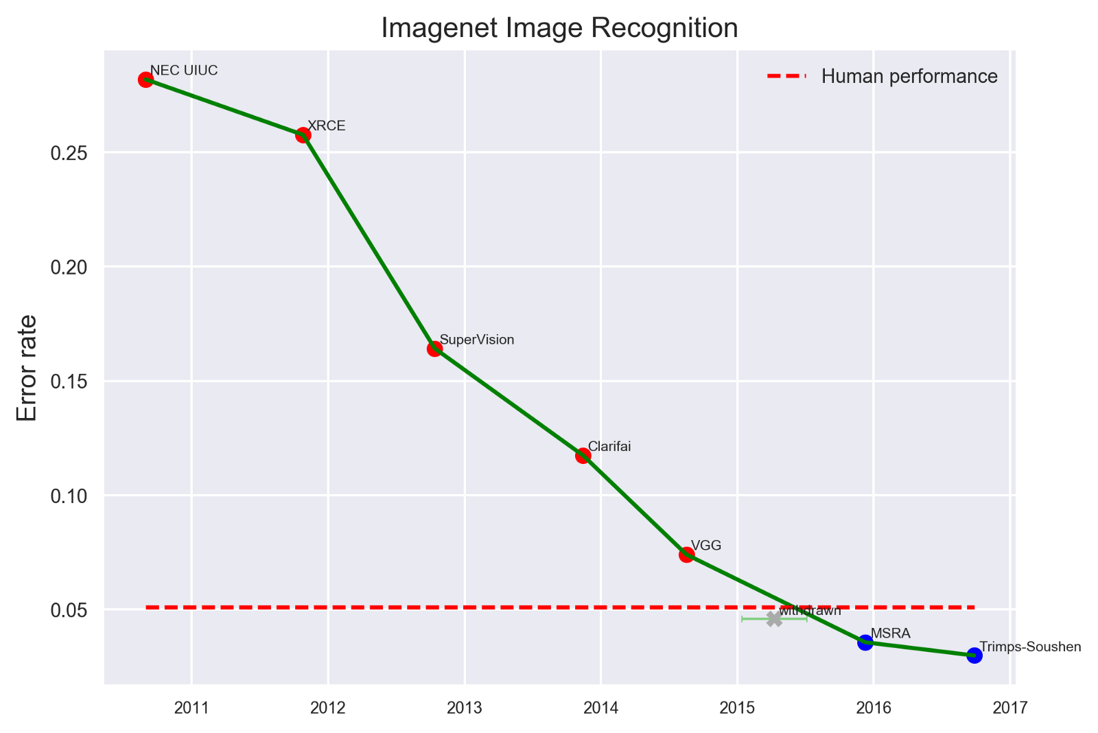
image source：https://www.eff.org/ai/metrics

• 1
• 2

如果想克服收集数以千计的训练图像的高昂费用，图像增强则就是从现有数据集生成训练数据。 
图像增强是将已经存在于训练数据集中的图像进行处理，并对其进行处理以创建相同图像的许多改变的版本。

这既提供了更多的图像来训练，也可以帮助我们的分类器暴露在更广泛的俩个都和色彩情况下，从而使我们的分类器更具有鲁棒性，以下是imgaug库中不同增强的一些示例

source image:https://github.com/aleju/imgaug

2.使用Keras进行基本图像增强

有很多方法来预处理图像，在这篇文章中，我借鉴使用keras深度学习库为增强图像提供的一些最常用的开箱即用方法，然后演示如何修改keras.preprocessing image.py文件以启用直方图均衡化方法。

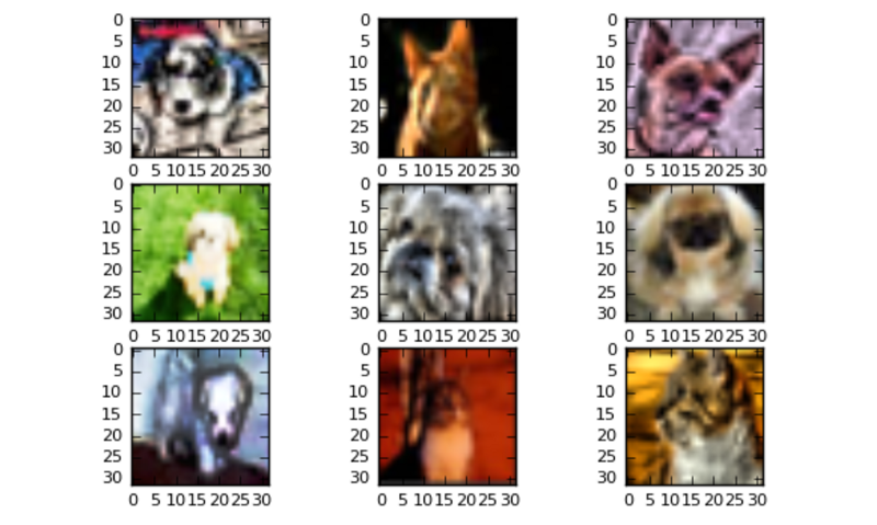
我们将使用keras自带的cifar10数据集。但是，我们只会使用数据集中的猫和狗的图像，以便保持足够小的任务在CPU上执行。

• 加载 和 格式化数据

我们要做的第一件事就是加载cifar10数据集并格式化图像，为CNN做准备。 
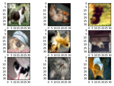
我们还会仔细查看一些图像，以确保数据已正确加载

先偷看一下长什么样？

16]:
from __future__ import print_function
import keras
from keras.datasets import cifar10
from keras import backend as K
import matplotlib
from matplotlib import pyplot as plt
import numpy as np# input image dimensions
img_rows, img_cols = 32, 32   # the data, shuffled and split between train and test sets
(x_train, y_train), (x_test, y_test) = cifar10.load_data()   # Only look at cats [=3] and dogs [=5]
train_picks = np.ravel(np.logical_or(y_train==3,y_train==5))
test_picks = np.ravel(np.logical_or(y_test==3,y_test==5))     y_train = np.array(y_train[train_picks]==5,dtype=int)
y_test = np.array(y_test[test_picks]==5,dtype=int)x_train = x_train[train_picks]
x_test = x_test[test_picks]...
...
...images = range(0,9)for i in images:plt.subplot(330 + 1 + i)plt.imshow(x_train[i], cmap=pyplot.get_cmap('gray'))
# show the plot
plt.show()

• 1
• 2
• 3
• 4
• 5
• 6
• 7
• 8
• 9
• 10
• 11
• 12
• 13
• 14
• 15
• 16
• 17
• 18
• 19
• 20
• 21
• 22
• 23
• 24
• 25
• 26
• 27
• 28
• 29
• 30
• 31
• 32
• 33
• 34
• 35
• 36

此处代码参考链接地址：https://github.com/ryanleeallred/Image_Augmentation/blob/master/Histogram_Modification.ipynb

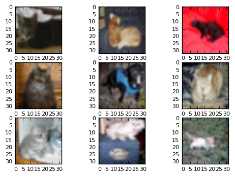
cifar10图像只有32 x 32像素，所以在这里放大时看起来有颗粒感，但是CNN并不知道它有颗粒感，只能看到数据, 嗯，还是人类牛逼。

• 从ImageDataGenerator（）创建一个图像生成器

用keras增强 图像数据 非常简单。 Jason Brownlee 对此提供了一个很好的教程。

首先，我们需要通过调用ImageDataGenerator()函数来创建一个图像生成器，并将它传递给我们想要在图像上执行的变化的参数列表。

然后，我们将调用fit()我们的图像生成器的功能，这将逐批地应用到图像的变化。默认情况下，这些修改将被随机应用，所以并不是每一个图像都会被改变。大家也可以使用keras.preprocessing导出增强的图像文件到一个文件夹，以便建立一个巨大的数据集的改变图像，如果你想这样做，可以参考keras文档。

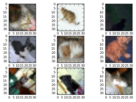
• 随机旋转图像

# Rotate images by 90 degrees
datagen = ImageDataGenerator(rotation_range=90)
# fit parameters from data
datagen.fit(x_train)
# Configure batch size and retrieve one batch of images
for X_batch, y_batch in datagen.flow(x_train, y_train, batch_size=9):# Show 9 imagesfor i in range(0, 9):pyplot.subplot(330 + 1 + i)pyplot.imshow(X_batch[i].reshape(img_rows, img_cols, 3))# show the plotpyplot.show()break

• 1
• 2
• 3
• 4
• 5
• 6
• 7
• 8
• 9
• 10
• 11
• 12
• 13

• 垂直翻转图像

# Flip images vertically
datagen = ImageDataGenerator(vertical_flip=True)
# fit parameters from data
datagen.fit(x_train)
# Configure batch size and retrieve one batch of images
for X_batch, y_batch in datagen.flow(x_train, y_train, batch_size=9):# Show 9 imagesfor i in range(0, 9):pyplot.subplot(330 + 1 + i)pyplot.imshow(X_batch[i].reshape(img_rows, img_cols, 3))# show the plotpyplot.show()break

• 1
• 2
• 3
• 4
• 5
• 6
• 7
• 8
• 9
• 10
• 11
• 12
• 13
• 14

备注：我感觉这里需要针对数据集，因为很少有人把狗翻过来看，或者拍照（hahhhh）

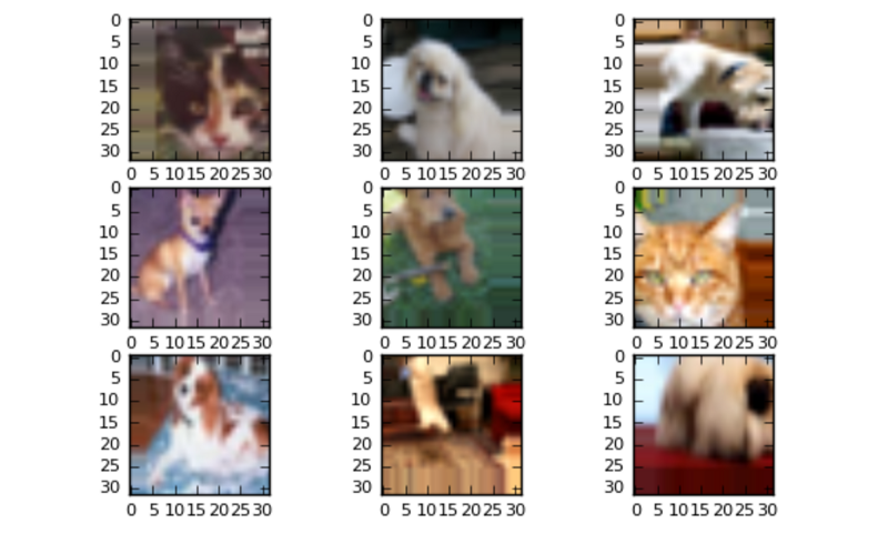
• 将图像垂直或水平移动20％

# Shift images vertically or horizontally
# Fill missing pixels with the color of the nearest pixel
datagen = ImageDataGenerator(width_shift_range=.2, height_shift_range=.2,fill_mode='nearest')
# fit parameters from data
datagen.fit(x_train)
# Configure batch size and retrieve one batch of images
for X_batch, y_batch in datagen.flow(x_train, y_train, batch_size=9):# Show 9 imagesfor i in range(0, 9):pyplot.subplot(330 + 1 + i)pyplot.imshow(X_batch[i].reshape(img_rows, img_cols, 3))# show the plotpyplot.show()break

• 1
• 2
• 3
• 4
• 5
• 6
• 7
• 8
• 9
• 10
• 11
• 12
• 13
• 14
• 15
• 16
• 17

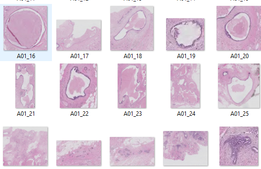
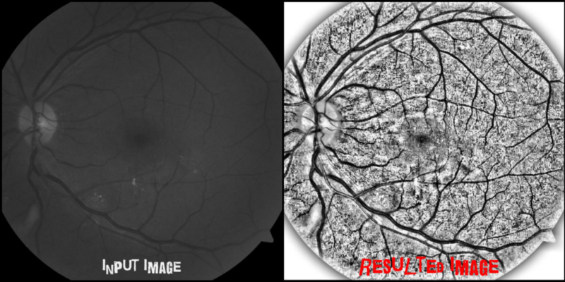
3.直方图均衡技术

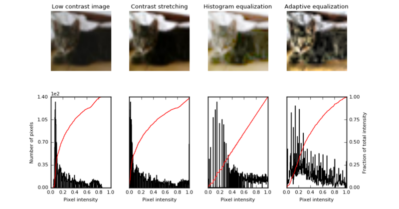
直方图均衡化是指对比度较低的图像，并增加图像相对高低的对比度，以便在阴影中产生细微的差异，并创建较高的对比度图像。结果可能是惊人的，特别是对于灰度图像,如图

使用图像增强技术来提高图像的对比度，此方法有时也被称为“ 直方图拉伸 
”，因为它们采用像素强度的分布和拉伸分布来适应更宽范围的值，从而增加图像的最亮部分和最暗部分之间的对比度水平。

直方图均衡 
直方图均衡通过检测图像中像素密度的分布并将这些像素密度绘制在直方图上来增加图像的对比度。然后分析该直方图的分布，并且如果存在当前未被使用的像素亮度范围，则直方图被“拉伸”以覆盖这些范围，然后被“ 
反投影 ”到图像上以增加总体形象的对比

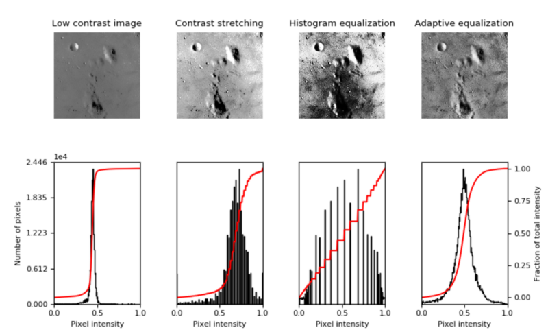
自适应均衡 
自适应均衡与常规直方图均衡的不同之处在于计算几个不同的直方图，每个直方图对应于图像的不同部分; 
然而，在其他无趣的部分有过度放大噪声的倾向。

下面的代码来自于sci-kit图像库的文档，并且已经被修改为在我们的cifar10数据集的第一个图像上执行上述三个增强。

首先，我们将从sci-kit图像（skimage）库中导入必要的模块，然后修改sci-kit图像文档中的代码以查看数据集第一幅图像上的增强

# Import skimage modules
from skimage import data, img_as_float
from skimage import exposure
# Lets try augmenting a cifar10 image using these techniques
from skimage import data, img_as_float
from skimage import exposure
# Load an example image from cifar10 dataset
img = images[0]
# Set font size for images
matplotlib.rcParams['font.size'] = 8
# Contrast stretching
p2, p98 = np.percentile(img, (2, 98))
img_rescale = exposure.rescale_intensity(img, in_range=(p2, p98))
# Histogram Equalization
img_eq = exposure.equalize_hist(img)
# Adaptive Equalization
img_adapteq = exposure.equalize_adapthist(img, clip_limit=0.03)
#### Everything below here is just to create the plot/graphs ####
# Display results
fig = plt.figure(figsize=(8, 5))
axes = np.zeros((2, 4), dtype=np.object)
axes[0, 0] = fig.add_subplot(2, 4, 1)
for i in range(1, 4):axes[0, i] = fig.add_subplot(2, 4, 1+i, sharex=axes[0,0], sharey=axes[0,0])
for i in range(0, 4):axes[1, i] = fig.add_subplot(2, 4, 5+i)
ax_img, ax_hist, ax_cdf = plot_img_and_hist(img, axes[:, 0])
ax_img.set_title('Low contrast image')
y_min, y_max = ax_hist.get_ylim()
ax_hist.set_ylabel('Number of pixels')
ax_hist.set_yticks(np.linspace(0, y_max, 5))
ax_img, ax_hist, ax_cdf = plot_img_and_hist(img_rescale, axes[:, 1])
ax_img.set_title('Contrast stretching')
ax_img, ax_hist, ax_cdf = plot_img_and_hist(img_eq, axes[:, 2])
ax_img.set_title('Histogram equalization')
ax_img, ax_hist, ax_cdf = plot_img_and_hist(img_adapteq, axes[:, 3])
ax_img.set_title('Adaptive equalization')
ax_cdf.set_ylabel('Fraction of total intensity')
ax_cdf.set_yticks(np.linspace(0, 1, 5))
# prevent overlap of y-axis labels
fig.tight_layout()
plt.show()

• 1
• 2
• 3
• 4
• 5
• 6
• 7
• 8
• 9
• 10
• 11
• 12
• 13
• 14
• 15
• 16
• 17
• 18
• 19
• 20
• 21
• 22
• 23
• 24
• 25
• 26
• 27
• 28
• 29
• 30
• 31
• 32
• 33
• 34
• 35
• 36
• 37
• 38
• 39
• 40
• 41
• 42

4.修改keras.preprocessing以启用直方图均衡技术。

现在我们已经成功地从cifar10数据集中修改了一个图像，我们将演示如何修改keras.preprocessing 
image.py文件，以执行这些不同的直方图修改技术，就像我们开箱即可使用的keras增强使用ImageDataGenerator()。

以下是我们将要执行此功能的一般步骤：

• 在你自己的机器上找到keras.preprocessing image.py文件。
• 将image.py文件复制到您的文件或笔记本中。
• 为每个均衡技术添加一个属性到DataImageGenerator（）init函数。
• 将IF语句子句添加到random_transform方法，以便在我们调用时实现增强datagen.fit()。

对keras.preprocessing

image.py文件进行修改的最简单方法之一就是将其内容复制并粘贴到我们的代码中。这将删除需要导入它。为了确保您抓取的是之前导入的文件的相同版本，最好抓取image.py您计算机上已有的文件。 
运行print(keras.__file__)将打印出机器上keras库的路径。路径（对于mac用户）可能如下所示：

/usr/local/lib/python3.5/dist-packages/keras/__init__.pyc

• 1
• 2

这给了我们在本地机器上keras的路径。

继续前进，在那里导航，然后进入preprocessing文件夹。在里面preprocessing你会看到image.py文件。然后您可以将其内容复制到您的代码中。该文件很长，但对于初学者来说，这可能是最简单的方法之一。

编辑 image.py

在image.py的顶部，你可以注释掉这行：from ..import backend as K如果你已经包含在上面。

此时，请仔细检查以确保您正在导入必要的scikit-image模块，以便复制的模块image.py可以看到它们。

from skimage import data, img_as_float
from skimage import exposure

• 1
• 2
• 3

我们现在需要在ImageDataGenerator类的 _ init _ 
方法中添加六行代码，以便它具有三个代表我们要添加的增强类型的属性。下面的代码是从我目前的image.py中复制的。与#####侧面的线是我已经添加的线

def __init __（self，
contrast_stretching = False，#####
histogram_equalization = False，#####
adaptive_equalization = False，#####
featurewise_center = False，
samplewise_center = False，
featurewise_std_normalization = False，
samplewise_std_normalization = False，
zca_whitening =假，
rotation_range = 0，
width_shift_range = 0，
height_shift_range = 0，
shear_range = 0，
zoom_range = 0，
channel_shift_range = 0，
fill_mode ='nearest'，
cval = 0，
horizo​​ntal_flip = False，
vertical_flip = False ，rescale
= None，
preprocessing_function = None，
data_format = None）：
if data_format is None：
data_format = K.image_data_format（）
self.counter = 0
self.contrast_stretching = contrast_stretching，#####
self.adaptive_equalization = adaptive_equalization #####
self.histogram_equalization = histogram_equalization #####
self.featurewise_center = featurewise_center
self。 samplewise_center = samplewise_center
self.featurewise_std_normalization = featurewise_std_normalization
self.samplewise_std_normalization = samplewise_std_normalization
self.zca_whitening = zca_whitening
self.rotation_range = rotation_range
self.width_shift_range = width_shift_range
self.height_shift_range = height_shift_range
self.shear_range = shear_range
self.zoom_range = zoom_range
self.channel_shift_range = channel_shift_range
self.fill_mode = fill_mode
self.cval = cval
self.horizo​​ntal_flip = horizo​​ntal_flip
self.vertical_flip = vertical_flip
self.rescale =
rescale self.preprocessing_function = preprocessing_function

• 1
• 2
• 3
• 4
• 5
• 6
• 7
• 8
• 9
• 10
• 11
• 12
• 13
• 14
• 15
• 16
• 17
• 18
• 19
• 20
• 21
• 22
• 23
• 24
• 25
• 26
• 27
• 28
• 29
• 30
• 31
• 32
• 33
• 34
• 35
• 36
• 37
• 38
• 39
• 40
• 41
• 42
• 43
• 44
• 45

该random_transform()（下）函数来响应我们一直传递到的参数ImageDataGenerator()功能。

如果我们已经设置了contrast_stretching，adaptive_equalization或者histogram_equalization参数True，当我们调用ImageDataGenerator()时（就像我们对其他图像增强一样）random_transform()将会应用所需的图像增强。

def random_transform(self, x):img_row_axis = self.row_axis - 1img_col_axis = self.col_axis - 1img_channel_axis = self.channel_axis - 1
# use composition of homographies
# to generate final transform that needs to be appliedif self.rotation_range:theta = np.pi / 180 * np.random.uniform(-self.rotation_range, self.rotation_range)else:theta = 0if self.height_shift_range:tx = np.random.uniform(-self.height_shift_range, self.height_shift_range) * x.shape[img_row_axis]else:tx = 0if self.width_shift_range:ty = np.random.uniform(-self.width_shift_range, self.width_shift_range) * x.shape[img_col_axis]else:ty = 0if self.shear_range:shear = np.random.uniform(-self.shear_range, self.shear_range)else:shear = 0if self.zoom_range[0] == 1 and self.zoom_range[1] == 1:zx, zy = 1, 1else:zx, zy = np.random.uniform(self.zoom_range[0], self.zoom_range[1], 2)
transform_matrix = Noneif theta != 0:rotation_matrix = np.array([[np.cos(theta), -np.sin(theta), 0],[np.sin(theta), np.cos(theta), 0],[0, 0, 1]])transform_matrix = rotation_matrixif tx != 0 or ty != 0:shift_matrix = np.array([[1, 0, tx],[0, 1, ty],[0, 0, 1]])transform_matrix = shift_matrix if transform_matrix is None else np.dot(transform_matrix, shift_matrix)if shear != 0:shear_matrix = np.array([[1, -np.sin(shear), 0],[0, np.cos(shear), 0],[0, 0, 1]])transform_matrix = shear_matrix if transform_matrix is None else np.dot(transform_matrix, shear_matrix)if zx != 1 or zy != 1:zoom_matrix = np.array([[zx, 0, 0],[0, zy, 0],[0, 0, 1]])transform_matrix = zoom_matrix if transform_matrix is None else np.dot(transform_matrix, zoom_matrix)if transform_matrix is not None:h, w = x.shape[img_row_axis], x.shape[img_col_axis]transform_matrix = transform_matrix_offset_center(transform_matrix, h, w)x = apply_transform(x, transform_matrix, img_channel_axis,fill_mode=self.fill_mode, cval=self.cval)if self.channel_shift_range != 0:x = random_channel_shift(x, self.channel_shift_range, img_channel_axis)if self.horizontal_flip:if np.random.random() < 0.5:x = flip_axis(x, img_col_axis)if self.vertical_flip:if np.random.random() < 0.5:x = flip_axis(x, img_row_axis)if self.contrast_stretching: #####if np.random.random() < 0.5: #####p2, p98 = np.percentile(x, (2, 98)) #####x = exposure.rescale_intensity(x, in_range=(p2, p98)) #####if self.adaptive_equalization: #####if np.random.random() < 0.5: #####x = exposure.equalize_adapthist(x, clip_limit=0.03) #####if self.histogram_equalization: #####if np.random.random() < 0.5: #####x = exposure.equalize_hist(x) #####return x

• 1
• 2
• 3
• 4
• 5
• 6
• 7
• 8
• 9
• 10
• 11
• 12
• 13
• 14
• 15
• 16
• 17
• 18
• 19
• 20
• 21
• 22
• 23
• 24
• 25
• 26
• 27
• 28
• 29
• 30
• 31
• 32
• 33
• 34
• 35
• 36
• 37
• 38
• 39
• 40
• 41
• 42
• 43
• 44
• 45
• 46
• 47
• 48
• 49
• 50
• 51
• 52
• 53
• 54
• 55
• 56
• 57
• 58
• 59
• 60
• 61
• 62
• 63
• 64
• 65
• 66
• 67
• 68
• 69
• 70
• 71
• 72
• 73
• 74
• 75

现在我们拥有所有必要的代码，并且可以调用ImageDataGenerator（）来执行我们的直方图修改技术。如果我们将所有三个值都设置为，则这是几张图片的样子True

# Initialize Generator
datagen = ImageDataGenerator(contrast_stretching=True, adaptive_equalization=True, histogram_equalization=True)
# fit parameters from data
datagen.fit(x_train)
# Configure batch size and retrieve one batch of images
for x_batch, y_batch in datagen.flow(x_train, y_train, batch_size=9):# Show the first 9 imagesfor i in range(0, 9):pyplot.subplot(330 + 1 + i)pyplot.imshow(x_batch[i].reshape(img_rows, img_cols, 3))# show the plotpyplot.show()break

• 1
• 2
• 3
• 4
• 5
• 6
• 7
• 8
• 9
• 10
• 11
• 12
• 13

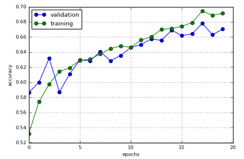
• 培训并验证您的Keras CNN

最后一步是训练CNN并验证模型model.fit_generator()，以便在增强图像上训练和验证我们的神经网络.

from keras.models import Sequential
from keras.layers import Dense, Dropout, Flatten
from keras.layers import Conv2D, MaxPooling2D
batch_size = 64
num_classes = 2
epochs = 10
model = Sequential()
model.add(Conv2D(4, kernel_size=(3, 3),activation='relu',input_shape=input_shape))
model.add(Conv2D(8, (3, 3), activation='relu'))
model.add(MaxPooling2D(pool_size=(2, 2)))
model.add(Dropout(0.25))
model.add(Flatten())
model.add(Dense(16, activation='relu'))
model.add(Dropout(0.5))
model.add(Dense(2, activation='softmax'))model.compile(loss=keras.losses.categorical_crossentropy,optimizer=keras.optimizers.Adadelta(),metrics=['accuracy'])
datagen.fit(x_train)
history = model.fit_generator(datagen.flow(x_train, y_train, batch_size=batch_size),steps_per_epoch=x_train.shape[0] // batch_size,epochs=20,validation_data=(x_test, y_test))

• 1
• 2
• 3
• 4
• 5
• 6
• 7
• 8
• 9
• 10
• 11
• 12
• 13
• 14
• 15
• 16
• 17
• 18
• 19
• 20
• 21
• 22
• 23
• 24

End 总结

这是我最后的测试结果

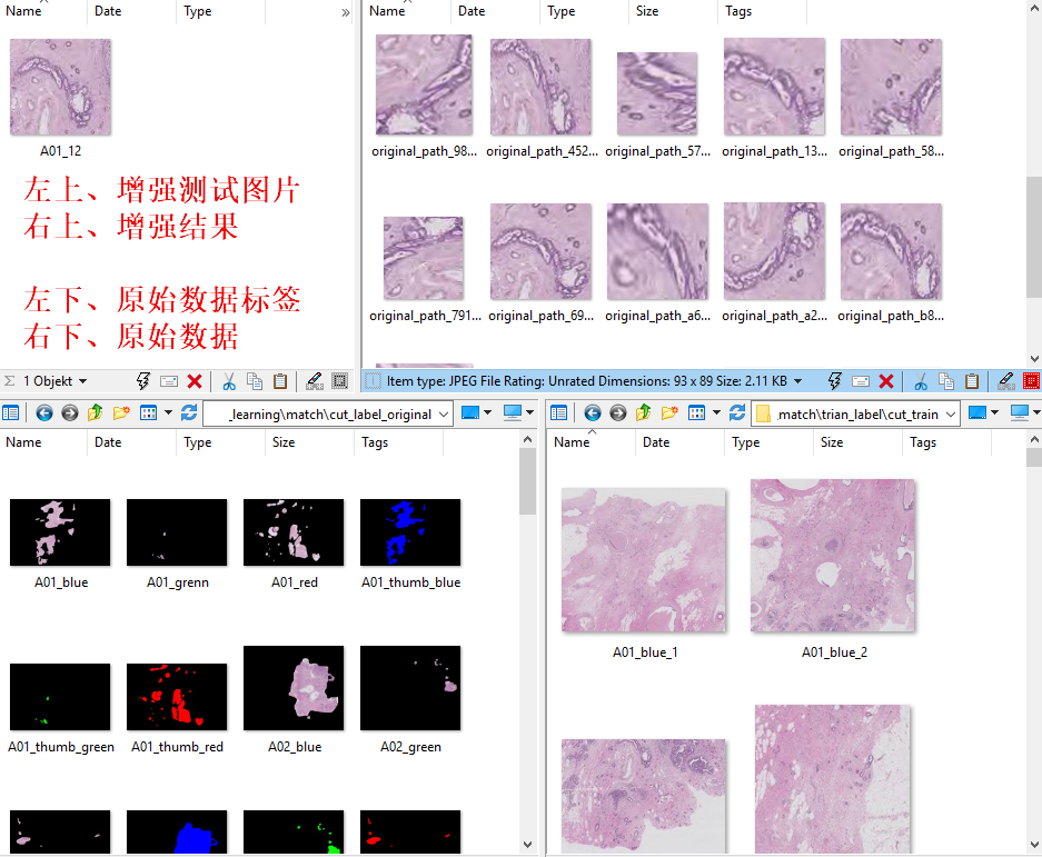
左上、增强测试图片 右上、增强结果

左下、原始数据标签 右下、原始数据

大家自己尝试一下哈，加油！