Machine learning, together with many other advanced data processing paradigms, fits incredibly well to the parallel-processing architecture that GPU computing offers.

机器学习以及许多其他高级数据处理范例非常适合GPU计算提供的并行处理架构。

In this article you’ll learn how to write your own ML algorithm from scratch in GPU optimized code, which will be able to run in virtually any hardware — including your mobile phone. We’ll introduce core GPU & ML concepts and show how you can use the Kompute framework to implement it in only a handful lines of code.

在本文中，您将学习如何在GPU优化的代码中从头开始编写自己的ML算法，该代码几乎可以在任何硬件(包括手机)中运行。 我们将介绍GPU和ML的核心概念，并展示如何使用Kompute框架仅用少量代码来实现它。

We will be building first a simple algorithm that will multiply two arrays in parallel, which will introduce the fundamentals of GPU processing. We will then write a Logistic Regression algorithm from scratch in the GPU. You can find the repo with the full code in the following links:

我们将首先构建一个简单的算法，该算法将两个数组并行相乘，从而介绍GPU处理的基本原理。 然后，我们将从头开始在GPU中编写Logistic回归算法。 您可以在以下链接中找到包含完整代码的仓库：

• Vulkan Kompute Repository

  Vulkan Kompute存储库

• GPU Array Multiplication Repository and Kompute Code

  GPU阵列乘法存储库和Kompute代码

• GPU Logistic Regression Repository, Kompute Code and Shader Code

  GPU Logistic回归存储库 ， Kompute代码和着色器代码

动机 (Motivation)

The potential and adoption of GPU computing has been exploding in recent years — you can get a glimps of the increasing speed in adoption from the charts in the image below. In deep learning there has been a massive increase in adoption of GPUs for processing, together with paradigms that have enabled massively parallelizable distribution of compute tasks across increasing number of GPU nodes. There is a lot of exciting research around techniques that propose new approaches towards model parallelism and data parallelism— both which allow algorithms and data respectively to be sub-divided in a broad range of approaches to maximize processing efficiency.

近年来，GPU计算的潜力和采用率一直在爆炸式增长-您可以从下图中的图表中快速了解采用率的提高速度。 在深度学习中，GPU在处理方面的采用已大大增加，而范式已使跨越来越多的GPU节点实现大规模可并行化的计算任务分配。 关于技术的提议，有很多令人兴奋的研究，它们提出了针对模型并行性和数据并行性的新方法，它们都允许将算法和数据分别细分为多种方法，以最大化处理效率。

In this article we outline the theory, and hands on tools that will enable both, beginners and seasoned GPU compute practitioners, to be make use of and contribute to the current development and discussions across these fascinating high performance computing areas.

在本文中，我们概述了该理论，并提供了动手工具，使初学者和经验丰富的GPU计算从业人员都可以利用并为这些引人入胜的高性能计算领域中的当前开发和讨论做出贡献。

Vulkan框架 (The Vulkan Framework)

Before diving right in, it’s worth introducing the core framework that is making it possible to build hyper-optimized, cross platform and scalable GPU algorithms — and that is the Vulkan Framework.

在深入研究之前，值得介绍一下核心框架，该框架使构建超级优化的跨平台和可扩展的GPU算法成为可能，这就是Vulkan框架。

Vulkan is an Open Source project led by the Khronos Group, a consortium of a very large number of tech companies who have come together to work towards defining and advancing the open standards for mobile and desktop media (and compute) technologies. On the left you can see the broad range of Khronos Members.

Vulkan是一个由Khronos Group领导的开源项目， Khronos Group是由许多技术公司组成的财团，它们共同致力于为移动和桌面媒体(和计算)技术定义和推进开放标准。 在左侧，您可以看到各种各样的Khronos会员。

You may be wondering, why do we need yet another new GPU framework where there are already many options available for writing parallelizable GPU code? The main reason is that unlike some of its closed source counterparts (e.g. NVIDIA’s CUDA, or Apple’s Metal) Vulkan is fully Open Source, and unlike some of the older options (e.g. OpenGL), Vulkan is built with the modern GPU architecture in mind, providing very granular access to GPU optimizations. Finally, whilst some alternatives provide vendor-specific support for GPUs, Vulkan provides cross-platform, and cross-vendor support, which means that it opens the doors to opportunities in mobile processing, edge computing, and more.

您可能想知道， 为什么我们还需要一个新的GPU框架，其中已经有很多选项可用于编写可并行化的GPU代码？ 主要原因是，Vulkan与某些封闭源同类产品(例如NVIDIA的CUDA或Apple的Metal)不同，它是完全开源的，与某些旧选项(如OpenGL)不同的是，Vulkan的构建考虑了现代GPU架构，提供对GPU优化的非常细粒度的访问。 最后，虽然某些替代方案为GPU提供了特定于供应商的支持，但Vulkan提供了跨平台和跨供应商的支持，这意味着它为移动处理，边缘计算等方面的商机打开了大门。

Vulkan’s C-API also provides very low level access to GPUs, which allows for very specialized optimizations. This is a great asset for GPU developers — the main disadvantage is the verbosity involved, requiring 500–2000+ lines of code to only get the base boilerplate required to even start writing the application logic. This can result not only in expensive developer cycles but also prone to small errors that can lead to larger problems.

Vulkan的C-API还提供了对GPU的低级访问，从而可以进行非常专业的优化。 对于GPU开发人员而言，这是一笔巨大的财富-主要缺点是涉及冗长，需要500-2000多行代码才能获得甚至开始编写应用程序逻辑所需的基础样板。 这不仅会导致昂贵的开发人员周期，而且容易产生小的错误，从而导致更大的问题。

输入Vulkan Kompute (Enter Vulkan Kompute)

Vulkan Kompute is a framework built on top of the Vulkan SDK, specifically designed to extend its compute capabilities as a simple to use, highly optimized, and mobile friendly General Purpose GPU computing framework.

Vulkan Kompute是在Vulkan SDK之上构建的框架，专门设计用于扩展其计算功能，使其成为易于使用，高度优化和移动友好的通用GPU计算框架。

Kompute was not built to hide any of the core Vulkan concepts — the Vulkan API is very well designed —instead it augments Vulkan’s Computing capabilities with a BYOV (bring your own Vulkan) design, enabling developers by reducing boilerplate code required and automating some of the more common workflows involved in writing Vulkan applications.

Kompute并不是为了隐藏Vulkan的任何核心概念而设计的-Vulkan API的设计非常好-而是通过BYOV(自带Vulkan)设计增强了Vulkan的计算功能，从而通过减少所需的样板代码并使某些功能自动化来使开发人员能够使用编写Vulkan应用程序涉及的更常见的工作流程。

For new developers curious to learn more, it provides a solid base to get started into GPU computing. For more advanced Vulkan developers, Kompute allows them to integrate it into their existing Vulkan applications, and perform very granular optimizations by getting access to all of the Vulkan internals when required. The project is fully open source, and we welcome bug reports, documentation extensions, new examples or suggestions — please feel free to open an issue in the repo.

对于渴望了解更多信息的新开发人员，它为入门GPU计算提供了坚实的基础。 对于更高级的Vulkan开发人员，Kompute允许他们将其集成到现有的Vulkan应用程序中，并通过在需要时访问所有Vulkan内部组件来执行非常精细的优化。 该项目是完全开源的，我们欢迎错误报告，文档扩展，新示例或建议-请随时在存储库中打开一个问题 。

写你的第一个Kompute (Writing your first Kompute)

To build our first simple array-multiplication GPU computing application using Kompute, we will create the following:

为了使用Kompute构建我们的第一个简单的数组乘法GPU计算应用程序，我们将创建以下代码：

• Two Kompute Tensors to store the input data

  两个Kompute张量存储输入数据

• One Kompute Tensor to store the output data

  一个Kompute张量来存储输出数据

• A Kompute Operation to create and copy the tensors to the GPU

  Kompute操作以创建张量并将其复制到GPU

• A Kompute Operation with an Kompute Algorithm that will hold the code to be executed in the GPU (called a “shader”)

  具有Kompute算法的Kompute操作 ，该操作将保存要在GPU中执行的代码(称为“着色器”)

• A Kompute Operation to sync the GPU data back to the local tensors

  Kompute操作将GPU数据同步回本地张量

• A Kompute Sequence to record the operations to send to the GPU in batches (we’ll use the Kompute Manager to simplify the workflow)

  Kompute序列，用于记录要批量发送到GPU的操作(我们将使用Kompute Manager简化工作流程)

At the core of Vulkan Kompute are “Kompute Operations”, which are used for GPU actions, as well as “Kompute Tensor” operations to handle the GPU data and memory. More specifically, this diagram shows the relationship between Kompute components (including explicit memory ownership).

Vulkan Kompute的核心是用于GPU操作的“ Kompute操作”，以及用于处理GPU数据和内存的“ Kompute Tensor”操作。 更具体地说，此图显示了Kompute组件之间的关系(包括显式的内存所有权)。

When interacting with the GPU, you have to send the instructions to the GPU to execute, and you need to make sure that the GPU has all of the relevant data available in GPU memory to begin processing. With Vulkan you send these instructions to the GPU via a queue, so to simplify things intuitively you can think of your GPU as a remote server, where data serialization, resource creation and memory allocation is expensive, and instructions are submitted via a queue — there is still GPU-CPU shared memory but you tend to only use this for data transfer to the GPU.

与GPU交互时，您必须将指令发送给GPU才能执行，并且需要确保GPU在GPU内存中具有所有可用的相关数据才能开始处理。 使用Vulkan，您可以通过队列将这些指令发送到GPU，因此，为了直观地简化操作，您可以将GPU视为远程服务器，其中数据序列化，资源创建和内存分配非常昂贵，并且指令是通过队列提交的–仍然是GPU-CPU共享内存，但是您倾向于仅将其用于将数据传输到GPU。

Let’s jump into the code. Typically in a Kompute application we’ll follow the following steps:

让我们跳入代码。 通常，在Kompute应用程序中，我们将遵循以下步骤：

1. Create a Kompute Manager to manage resources创建Kompute Manager来管理资源
2. Create Kompute Tensors to hold data创建Kompute张量来保存数据
3. Initialise the Kompute Tensors in the GPU with a Kompute Operation使用Kompute操作在GPU中初始化Kompute张量
4. Define the code to run on the GPU as a “compute shader”定义要在GPU上运行的代码作为“计算着色器”
5. Use Kompute Operation to run shader against Kompute Tensors使用Kompute Operation对Kompute张量运行着色器
6. Use Kompute Operation to map GPU output data into local Tensors使用Kompute Operation将GPU输出数据映射到本地张量
7. Print your results打印结果

1.创建一个Kompute Manager来管理资源 (1. Create a Kompute Manager to manage resources)

First, we’ll create our Kompute Manager, which is in charge of creating and managing all the underlying Vulkan resources.

首先，我们将创建Kompute Manager，它负责创建和管理所有基础Vulkan资源。

// Single header include for Kompute
#include "kompute/Kompute.hpp"int main() {// Vulkan resources get created unless passedkp::Manager mgr(0); // Selects GPU device at index 0//... continued in next section
}

As you can see, here we are initializing our Kompute Manager, expecting it to create all the base Vulkan resources on Device 0 (in my case Device 0 is my NVIDIA card, and Device 1 is my integrated graphics card). For more advanced use-cases it’s also possible to initialize the Kompute Manager with your own Vulkan resources (Device, Queue, etc) but this is out of scope of this article.

如您所见，这里我们正在初始化Kompute Manager，期望它在Device 0上创建所有基本Vulkan资源(在我的情况下，Device 0是我的NVIDIA卡，而Device 1是我的集成显卡)。 对于更高级的用例，还可以使用自己的Vulkan资源(设备，队列等)来初始化Kompute Manager，但这不在本文的讨论范围之内。

2.创建Kompute张量来保存数据 (2. Create Kompute Tensors to hold data)

We will now create the Kompute Tensors that will be used for input and output. These will hold the data required which will be mapped into the GPU to perform this simple multiplication.

现在，我们将创建将用于输入和输出的Kompute张量。 这些将保存所需的数据，这些数据将被映射到GPU中以执行此简单乘法。

int main()
{//... continued from previous sectionstd::shared_ptr<kp::Tensor> tensorInA{ new kp::Tensor({ 2.0, 4.0, 6.0 }) };std::shared_ptr<kp::Tensor> tensorInB{ new kp::Tensor({ 0.0, 1.0, 2.0 }) };std::shared_ptr<kp::Tensor> tensorOut{ new kp::Tensor({ 0.0, 0.0, 0.0 }) };//... continued in next section
}

The reason why Kompute uses std::shared_ptr by design to avoid passing the objects by value, and instead passing them using smart pointers.

Kompute故意使用std::shared_ptr来避免按值传递对象，而是使用智能指针传递对象的原因。

3.通过Kompute操作在GPU中初始化Kompute张量 (3. Initialise the Kompute Tensors in the GPU with a Kompute Operation)

Now that we have our Tensors created with local data, we will map the data into the GPU. For this we will use the kp::OpTensorCreate Kompute Operation, which will initialize the underlying Vulkan buffer and GPU memory, and perform the respective mapping into the GPU.

现在我们已经使用本地数据创建了Tensors，我们将数据映射到GPU中。 为此，我们将使用kp::OpTensorCreate Kompute操作，该操作将初始化基础Vulkan缓冲区和GPU内存，并执行到GPU的相应映射。

int main()
{//... continued from previous section// Create the tensors by passing them as parametersmgr.evalOpDefault<kp::OpTensorCreate>({ tensorInA, tensorInB, tensorOut });//... continued in next section
}

It’s also worth mentioning that it’s possible to shorten the tensor creation steps by leveraging the Kompute Manager buildTensor helper function. This would allow you to skip the need to create the shared_ptr explicitly as well as the kp::OpTensorCreate Operation as outlined below (you can also find the full code implementation of this variation here).

还值得一提的是，可以利用Kompute Manager buildTensor辅助函数来缩短张量创建步骤。 这将使您无需显式创建shared_ptr以及下面概述的kp::OpTensorCreate操作的需求(您也可以在此处找到此变体的完整代码实现)。

int main()
{//... continued from previous section// Using this instead of Operationsauto tensorInA = mgr.buildTensor({ 2.0, 4.0, 6.0 });auto tensorInB = mgr.buildTensor({ 0.0, 1.0, 2.0 });auto tensorOut = mgr.buildTensor({ 0.0, 0.0, 0.0 });//... continued in next section
}

4.定义要在GPU上运行的代码作为“计算着色器” (4. Define the code to run on the GPU as a “compute shader”)

Now that we’ve initialized the necessary Kompute Tensor components and they are mapped in GPU memory, we can add the Kompute Algorithm that will be executed in the GPU. This is referred to as the “shader” code, which follows a C-like syntax. You can see the full shader code below, and we’ll break down each of the sections below.

现在我们已经初始化了必要的Kompute Tensor组件并将它们映射到GPU内存中，我们可以添加将在GPU中执行的Kompute算法。 这被称为“着色器”代码，遵循类似C的语法。 您可以在下面看到完整的着色器代码，我们将细分下面的每个部分。

int main()
{//... continued from previous section// Define your shader as a string (using string literals for simplicity)// (You can also pass the raw compiled bytes, or even path to file)std::string shader(R"(// The version to use #version 450// The execution structurelayout (local_size_x = 1) in;// The buffers are provided via the tensorslayout(binding = 0) buffer bufA { float a[]; };layout(binding = 1) buffer bufB { float b[]; };layout(binding = 2) buffer bufOut { float o[]; };void main() {uint index = gl_GlobalInvocationID.x;o[index] = a[index] * b[index];})");//... continued in next section
}

The #version 450 and layout(local_size_x = 1) in; sections specify the version and parallel thread execution structure (which we’ll look at further down the article). We then can see the GPU data inputs and outputs defined in the format:

#version 450和layout(local_size_x = 1) in; 小节指定了版本和并行线程执行结构(我们将在本文的后面进一步介绍)。 然后，我们可以看到以以下格式定义的GPU数据输入和输出：

layout(binding = <INDEX>) buffer <UNIQUENAME> {float <VARNAME>[]};

layout(binding = <INDEX>) buffer <UNIQUENAME> {float <VARNAME>[]};

• <INDEX> — index that maps Tensors to the GPU input<INDEX> —将张量映射到GPU输入的索引
• <UNIQUENAME> — This has to just be a unique name for the buffer<UNIQUENAME>-这必须是缓冲区的唯一名称
• <VARNAME> — This is the variable name to use in the shader code<VARNAME> —这是在着色器代码中使用的变量名称

These are the parameters that can be used throughout the shader code for processing. Namely in this case, the processing is done inside the main function. The first variable uint index = gl_GlobalInvocationID.x; is the currently parallel execution index which will allow us to process each data input.

这些是可以在整个着色器代码中用于处理的参数。 即，在这种情况下，处理在main函数内部完成。 第一个变量uint index = gl_GlobalInvocationID.x; 是当前并行执行索引，它将使我们能够处理每个数据输入。

We then come into the core of this algorithm which is the multiplication o[index] = a[index] * b[index]. This part is quite self-explanatory — we multiply the elements of the GPU arrays a[] and b[] , then store the output on the array o[].

然后我们进入该算法的核心，即乘法o[index] = a[index] * b[index]. 这部分是不言自明的-我们将GPU数组a[]和b[]的元素相乘，然后将输出存储在数组o[] 。

5.使用Kompute Operation对Kompute张量运行着色器 (5. Use Kompute Operation to run shader against Kompute Tensors)

In order to run the shader above we will can the Kompute Operation kp::OpAlgoBase. The parameters required for this Kompute Operation includes the Tensors to bind into the GPU instructions, as well as the shader code itself.

为了运行上面的着色器，我们可以使用Kompute Operation kp::OpAlgoBase 。 此Kompute操作所需的参数包括绑定到GPU指令中的张量以及着色器代码本身。

int main()
{//... continued from previous section// Run Kompute operation on the Tensor parameters provided mgr.evalOpDefault<kp::OpAlgoBase<>>(tensorParams,std::vector<char>(shader.begin(), shader.end()));//... continued in next section
}

It’s worth mentioning that Kompute allows the user to also pass the shader through a file path, or alternative there are also Kompute tools that will allow you to convert the shader binaries into C++ header files.

值得一提的是，Kompute允许用户也通过文件路径传递着色器，或者，还有Kompute工具，可以将着色器二进制文件转换为C ++头文件。

6.使用Kompute Operation将GPU输出数据映射到本地张量 (6. Use Kompute Operation to map GPU output data into local Tensors)

Once the algorithm gets triggered, the result data will now held in the GPU memory of our output tensor. We can now use the kp::OpTensorSyncLocal Kompute Operation to sync the Tensor GPU memory as per the code block below.

触发算法后，结果数据现在将保存在输出张量的GPU内存中。 现在我们可以按照以下代码块使用kp::OpTensorSyncLocal Kompute操作来同步Tensor GPU内存。

int main()
{//... continued from previous section// Run Kompute operation on the parameters provided with dispatch layoutmgr.evalOpDefault<kp::OpTensorSyncLocal>({ tensorOut });//... continued in next section
}

7.打印结果 (7. Print your results)

Finally we can print the output data of our tensor.

最后，我们可以打印张量的输出数据。

int main()
{//... continued from previous section// prints "Output {  0  4  12  }"std::cout<< "Output: {  ";for (const float& elem : tensorOut->data()) {std::cout << elem << "  ";}std::cout << "}" << std::endl;
}

When you run this, you will see the values of your output tensor printed. That’s it, you’ve written your first Kompute!

运行此命令时，您将看到输出张量的值打印出来。 就是这样，您已经编写了第一本Kompute！

You can also find the full example in the repo so you can run it and extend it as desired. You can find the full standalone example in this repository which includes the instructions on how to build it as well as the Kompute C++ code.

您还可以在存储库中找到完整的示例，以便可以运行它并根据需要扩展它。 您可以在此存储库中找到完整的独立示例，其中包括有关如何构建它的说明以及Kompute C ++代码 。

Although it may not seem obvious, the above introduced some intuition around core concepts and design thinking in GPU computing, whilst still abstracting a couple of the more in-depth concepts. In the following sections we will be providing more concrete terminology and we’ll be scratching the surface of some of the more advanced concepts such as threads, blocks, memory strides and shared memory (although a lot will be provided as further reading).

尽管可能看起来并不明显，但以上内容介绍了一些有关GPU计算中核心概念和设计思想的直觉，同时仍然抽象出了一些更深入的概念。 在以下各节中，我们将提供更具体的术语，并且将介绍一些更高级的概念，例如线程，块，内存步幅和共享内存(尽管将提供许多内容供进一步阅读)。

深入研究机器学习的直觉 (Diving into the Machine Learning intuition)

Let’s look at a more advanced GPU compute use-case, specifically implementing the hello world of machine learning, logistic regression. Before we cover the implementation we will provide some intuition on the theory, and the terminology that we’ll be using throughout.

让我们看一个更高级的GPU计算用例，专门实现机器学习，逻辑回归的世界。 在介绍实现之前，我们将提供一些理论上的直觉，以及我们将在整个过程中使用的术语。

In machine learning we always have two stages, training and inference. In the diagram below you can see the two simplified flows. At the top is the training flow, where you identify some training data, extract some features, and train a model until you are happy with the accuracy. Once you have a trained model, you persist the model “weights” and deploy the model into the second workflow, where the model would perform inference on unseen data.

在机器学习中，我们总是有两个阶段，即训练和推理。 在下图中，您可以看到两个简化的流程。 训练流程位于顶部，您可以在其中识别一些训练数据，提取一些特征并训练模型，直到对准确性满意为止。 拥有训练有素的模型后，您将保留模型的“权重”并将其部署到第二个工作流程中，该模型将对看不见的数据进行推理。

In this case we will have an input dataset X , where each element is a pair xi and xj . Our input data will be the following:

在这种情况下，我们将有一个输入数据集X ，其中每个元素都是xi和xj对。 我们的输入数据如下：

• xi = { 0, 1, 1, 1, 1 }

  xi = { 0, 1, 1, 1, 1 }

• xj = { 0, 0, 0, 1, 1 }

  xj = { 0, 0, 0, 1, 1 }

WIth this input data, the expected target value Y to be predicted will be the following:

利用该输入数据，将要预测的预期目标值Y将为以下各项：

• Y = {0, 0, 0, 1, 1}

  Y = {0, 0, 0, 1, 1}

Our primary objective in machine learning is to learn using this data to find the function (and parameters) that will allow us to predict values Y from just using X as input.

我们机器学习的主要目标是学习使用这些数据来查找函数(和参数)，这些函数和参数将使我们仅使用X作为输入即可预测值Y

It’s worth noting that the predicted values are defined as ŷ , which are specifcially the values computed with our inference function, distinct to the “true” or “actual” values of Y that we defined above.

值得注意的是，预测值定义为ŷ ，特别是通过我们的推断函数计算出的值，与上面定义的Y的“真实”或“实际”值不同。

The functions that we will be using for logistic regression will be the following:

我们将用于逻辑回归的函数如下：

Let’s break down this function:

让我们分解一下这个功能：

• z — is our linear mapping function

  z —是我们的线性映射函数

• ŷ —is the resulting predicted outputs

  ŷ是预测的结果输出

• Xᵀ —The transpose of the matrix containing our inputs xi and xj

  X ᵀ-The含有我们的输入Xi和XJ矩阵的转置

• σ — The sigmoid function which is covered in more detail below

  σ S型函数，将在下面更详细地介绍

And the parameters that we’ll be looking to learn with our machine learning algorithm are:

我们希望通过机器学习算法学习的参数是：

• W— The weights that will be applied to the inputs

  W —将应用于输入的权重

• b — The bias that will be added

  b将会增加的偏见

There is also the surrounding function σ which is the sigmoid function. This function forces our input to be closer to 0 or 1, which could be intuitively seen as the probability of our prediction to be “true”, and is defined as following:

还有周围的函数σ ，它是S形函数。 此函数强制我们的输入接近0或1，可以直观地将其视为我们的预测为“ true”的概率，其定义如下：

This is now the inference function that will allow us to process predictions from new data points. If we say for example that we have a new unseen set of inputs X = { (0, 1) }, and we assume that the learned parameters were W = (1, 1), b = 0 after running our machine learning algorithm through our training data (which we’ll do later on), then we’ll be able to run this through our prediction function by substituting the values as follows:

现在，这就是推理功能，它将使我们能够处理来自新数据点的预测。 例如，如果我们说有一组新的看不见的输入X = { (0, 1) } ，并且我们假设通过运行我们的机器学习算法后W = (1, 1), b = 0学习到的参数为W = (1, 1), b = 0我们的训练数据(稍后我们将做)，然后我们可以通过将预测值替换为以下内容来通过我们的预测函数运行该数据：

In this case the prediction is 0.73..., which would be a positive prediction. This of course is just to demonstrate what our inference function will look like once we learn the parameters W and b.

在这种情况下，预测为0.73... ，这将是肯定的预测。 当然，这只是为了证明一旦学习了参数W和b. ，我们的推断函数将是什么样b.

The way that we will be learning the parameters is by performing a prediction, calculating the error, and then re-adjusting the weights accordingly. The method used to “re-adjust” the weights based on the “prediction error” will be done by leveraging gradient descent. This will be repeated multiple times to find more accurate parameters.

我们学习参数的方式是执行预测，计算误差，然后相应地重新调整权重。 基于“预测误差”来“重新调整”权重的方法将通过利用梯度下降来完成。 这将重复多次以找到更准确的参数。

For this we will need to use the derivatives of each of the formulas. The first one, which is the derivative of our linear mapping function z is:

为此，我们将需要使用每个公式的导数。 第一个是线性映射函数z的导数是：

• ∂z = z(x) - y∂z= z(x)-y

Where the variables are defined as follows:

变量定义如下：

• ∂z — The derivative of the linear mapping function z(x)

  ∂z线性映射函数z(x)

• z(x) — the result of the linear mapping function applied to input x

  z(x) —应用于输入x的线性映射函数的结果

• y — the actual value label expected for that input x

  y —该输入x的期望实际值标签

Similarly the derivatives for w and b respectively are the following:

类似地，w和b的导数分别如下：

• ∂w = (x - ∂z)/m∂w=(x-∂z)/ m
• ∂b = ∂z/m∂b=∂z/ m

In this case m is the total number of input elements.

在这种情况下， m是输入元素的总数。

We will now be able to re-adjust the parameters using the above as follows:

现在，我们可以使用上述方法重新调整参数，如下所示：

• w = w - θ · ∂ww = w-θ·∂w
• b = b - θ · ∂bb = b-θ·∂b

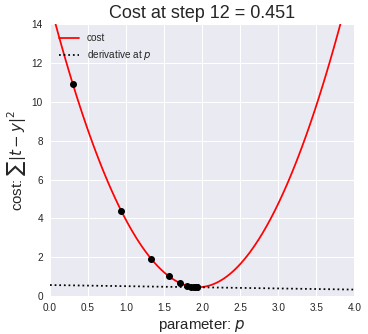
In this case θ is the learning rate, which as the name suggests controls the ratio by which the parameters will be modified on each iteration. Intuitively, the smaller, the more iterations it will be required for the algorithm to converge, however if the learning is too big, it will overshoot, leading to never being able to converge (from the image above you can imagine it will keep bouncing from side to side never reaching the bottom).

在这种情况下，θ是学习率，顾名思义，它控制着在每次迭代中修改参数的比率。 直观地讲，算法收敛所需的迭代次数越小，迭代次数就越多，但是，如果学习内容过多，则会导致过冲，从而导致永远无法收敛(从上图可以想象它会不断反弹并没有到达底部)。

In order for us to calculate loss, we will be using the log loss function, known also as cross-entropy loss function. This function is defined as follows:

为了计算损失，我们将使用对数损失函数，也称为交叉熵损失函数。 该函数定义如下：

The function itself is set up such that the larger the difference between the predicted class and the expected class, the larger the error (you can see how much it punishes if the predicted class is on the complete different label).

设置函数本身时，要使预测类和预期类之间的差异越大，则误差越大(您可以看到，如果预测类位于完全不同的标签上，则要付出多少代价)。

The loss function will provide us an idea of the improvement of our algorithm across iterations.

损失函数将为我们提供跨迭代改进算法的想法。

Finally, one of the most important points here will be the intuition behind how we can leverage the parallel architecture of the GPU to optimize computation. In this case, we’ll be able to do it by processing multiple input parameters at the same time, referred to as a micro-batch, and then re-adjusting the parameters in batch. This is known as data-parallelization, and is one of many techniques available. In the next section we will see how this is implemented, namely passing a mini-batch of inputs, storing the weights, and then re-adjusting them before the next iteration.

最后，这里最重要的要点之一就是我们如何利用GPU的并行体系结构来优化计算的直觉。 在这种情况下，我们可以通过同时处理多个输入参数(称为微批处理)并批量重新调整参数来做到这一点。 这称为数据并行化，并且是许多可用技术中的一种。 在下一节中，我们将了解如何实现此方法，即传递一个小批量输入，存储权重，然后在下一次迭代之前重新调整它们。

Note: In this post we won’t delve into much detail, nor best practices on machine learning, however at the end of the article we will be listing a broad range of sources for people interested to take their machine learning (or GPU compute) knowledge to the next level.

注意：在本文中，我们不会深入探讨机器学习的最佳细节，也不会介绍最佳实践，但是，在本文结尾，我们将为有兴趣进行机器学习(或GPU计算)的人们列出广泛的资源。知识到下一个层次。

机器学习GPU代码实现 (Machine Learning GPU Code Implementation)

Now that we have covered some of the core concepts, we will be able to learn about the implementation of the shader, which is the code that will be executed in the GPU.

现在，我们已经涵盖了一些核心概念，我们将能够了解着色器的实现，该着色器将在GPU中执行。

First we need to define all the input and output buffers as follows:

首先，我们需要定义所有输入和输出缓冲区，如下所示：

layout(set = 0, binding = 0) buffer bxi { float xi[]; };
layout(set = 0, binding = 1) buffer bxj { float xj[]; };
layout(set = 0, binding = 2) buffer by { float y[]; };
layout(set = 0, binding = 3) buffer bwin { float win[]; };
layout(set = 0, binding = 4) buffer bwouti { float wouti[]; };
layout(set = 0, binding = 5) buffer bwoutj { float woutj[]; };
layout(set = 0, binding = 6) buffer bbin { float bin[]; };
layout(set = 0, binding = 7) buffer bbout { float bout[]; };
layout(set = 0, binding = 8) buffer blout { float lout[]; };

If you remember, at the end of the last section we mentioned how we will be leveraging the concept of micro-batches in order to use the parallel architecture of GPU processing. What this means in practice, is that we will be passing multiple instances of X to the GPU to process at a time, instead of expecting the GPU to process it one by one. This is why we see that above we have an array for xi, xj, y, wOuti, wOutj, andbOut respectively.

如果您还记得的话，在上一节的最后，我们提到了如何利用微批处理的概念来使用GPU处理的并行体系结构。 实际上，这意味着我们将一次将多个X实例传递给GPU进行处理，而不是期望GPU一次处理它。 这就是为什么我们看到上面有一个分别用于xi, xj, y, wOuti, wOutj,和bOut 。

In more detail:

更详细地：

• The input X as arrays xi and xj will hold the micro-batch of inputs

  输入X作为数组xi和xj将保存输入的微批

• The array y will hold all the expected labels for micro-batch inputs

  数组y将保存微批输入的所有预期标签

• The two input weight parameters win will be used for calculating predictions

  输入的两个权重参数win将用于计算预测

• The input parameter b which will be used for calculating the predictions

  输入参数b将用于计算预测

• The output weights wouti and woutj contains weights and will store the derivative of W for all micro-batches that should be substracted

  输出权重wouti和woutj包含权重，并将存储所有应该减去的微批的W的导数

• Similarly the output bias array contains the derivatives of b for all micro-batches that should be substracted in batch

  类似地，输出偏置数组包含b的所有微批的b的导数。

• Finally lout contains the output array where losses will be returned

  最后lout包含输出数组，其中将返回损失

We also receive the constant M, which will be the total number of elements — if you remember this parameter will be used for the calculation of the derivatives. We will also see how these parameters are actually passed into the shader from the C++ Kompute side.

我们还收到常数M ，它是元素的总数-如果您还记得该参数将用于计算导数。 我们还将看到这些参数实际上是如何从C ++ Kompute端传递到着色器的。

layout (constant_id = 0) const uint M = 0;float m = float(M);

Now that we have all the input and output parameters defined, we can start the main function, which will contain the implementation of our machine learning training algorithm.

现在我们已经定义了所有输入和输出参数，我们可以启动main函数，它将包含我们的机器学习训练算法的实现。

We will first start by keeping track of the current index of the global invocation. Since the GPU executes in parallel, each of these runs will be running directly in parallel, so this allows the current execution to consistently keep track of what iteration index is currently being executed.

我们首先将从跟踪全局调用的当前索引开始。 由于GPU是并行执行的，因此这些运行中的每一个都将直接并行运行，因此这允许当前执行始终跟踪当前正在执行的迭代索引。

// ...code from previous blocksint main() {uint idx = gl_GlobalInvocationID.x;// ...code from latter blocks
}

We now can start preparing all the variables that we’ll be using throughout the algorithms. All our inputs are buffer arrays, so we’ll want to store them in vec2 and float variables.

现在，我们可以开始准备在整个算法中将要使用的所有变量。 我们所有的输入都是缓冲区数组，因此我们希望将它们存储在vec2和float变量中。

// ...code from previous blocksint main() {// ...code from previous blocksvec2 wCurr = vec2(win[0], win[1]);float bCurr = bin[0];vec2 xCurr = vec2(xi[idx], xj[idx]);float yCurr = y[idx];// ...code from latter blocks
}

In this case we’re basically making explicit the variables that are being used for the current “thread run”. The GPU architecture consists of slightly more nuanced execution structures that involve thread blocks, memory access limitations, etc — however we won’t be covering these in this example.

在这种情况下，我们基本上是在明确显示用于当前“线程运行”的变量。 GPU体系结构由稍微微妙的执行结构组成，这些执行结构涉及线程块，内存访问限制等，但是在本示例中我们将不介绍这些内容。

Now we get into the more fun part —implementing the inference function. Below we will implement the inference function to calculate ŷ, which involves both the linear mapping function, as well as the sigmoid function.

现在，我们进入更有趣的部分-实现推理功能。 下面我们将实现推论函数来计算ŷ，它既涉及线性映射函数，又涉及S形函数。

// ...code from previous blocksfloat sigmoid(float z) {return 1.0 / (1.0 + exp(-z));
}float inference(vec2 x, vec2 w, float b) {// Compute the linear mapping functionfloat z = dot(w, x) + b;// Calculate the y-hat with sigmoid float yHat = sigmoid(z);return yHat;
}int main() {// ...code from previous blocksfloat yHat = inference(xCurr, wCurr, bCurr);// ...code from latter blocks
}

Now that we have yHat, we can now use it to calculate the derivatives (∂z, ∂w and ∂b), which in this case are the derivative of the currently-executed index input element.

现在有了yHat ，我们现在可以使用它来计算导数(∂z，∂w和∂b)，在这种情况下，它们是当前执行的索引输入元素的导数。

// ...code from previous blocksint main() {// ...code from previous blocksfloat dZ = yHat - yCurr;vec2 dW = (1. / m) * xCurr * dZ;float dB = (1. / m) * dZ;// ...code from latter blocks
}

We can now pass the derivatives as outputs, so the parameters can be re-adjusted for the next iteration.

现在，我们可以将导数作为输出传递，因此可以为下一次迭代重新调整参数。

// ...code from previous blocksint main() {// ...code from previous blockswouti[idx] = dW.x;woutj[idx] = dW.y;bout[idx] = dB;// ...code from latter blocks
}

Finally we’re able to calculate the loss and add it to the output lout array.

最后，我们能够计算损失并将其添加到输出lout数组中。

// ...code from previous blocksfloat calculateLoss(float yHat, float y) {return -(y * log(yHat)  +  (1.0 - y) * log(1.0 - yHat));
}int main() {// ...code from previous blockslout[idx] = calculateLoss(yHat, yCurr);
}

That’s it, we’ve now finished the shader that will enable us to train a Logistic Regression algorithm in the GPU — you can find the full code for the shader in the GPU logistic regression example repository.

就这样，我们现在完成了着色器，使我们能够在GPU中训练Logistic回归算法-您可以在GPU Logistic回归示例存储库中找到着色器的完整代码 。

Now we’ll cover the Kompute code required to run this code against a dataset to train our first model and find the parameters.

现在，我们将介绍针对数据集运行此代码所需的Kompute代码，以训练我们的第一个模型并找到参数。

Kompute的机器学习编排 (Machine Learning Orchestration from Kompute)

In order to run the shader we created above in the GPU using Vulkan Kompute, we will follow the following steps:

为了使用Vulkan Kompute运行我们在GPU中上面创建的着色器，我们将遵循以下步骤：

1. Import Kompute and create our main function导入Kompute并创建我们的主要功能
2. Create all the Kompute Tensors required创建所需的所有Kompute张量
3. Create the Kompute Manager and initialize a Kompute Sequence创建Kompute Manager并初始化Kompute序列
4. Execute the Kompute Tensor GPU initialization via Kompute Sequence通过Kompute Sequence执行Kompute Tensor GPU初始化
5. Record batch algorithm execution in Kompute Sequence记录Kompute序列中的批处理算法执行
6. Iterate 100 times: Run micro-batch execution & update weights迭代100次：运行微批量执行并更新权重
7. Print resulting parameters to use for further inference打印结果参数以用于进一步推断

As you can see this is more involved than the simpler example we used above. In this case we will use the Kompute Sequence instead of the Kompute Manager directly, as we want to have deeper control on the commands that can be recorded to send in batch to the GPU. We will discuss this in more detail as we cover each of the steps. Let’s get started.

如您所见，这比我们上面使用的更简单的示例更复杂。 在这种情况下，我们将直接使用Kompute序列而不是Kompute Manager，因为我们希望对可记录以批量发送到GPU的命令进行更深入的控制。 在介绍每个步骤时，我们将对此进行更详细的讨论。 让我们开始吧。

1.导入Kompute并创建我们的主要功能 (1. Import Kompute and create our main function)

We will be importing the single header of Vulkan Kompute — it’s also possible to use the more granular class-based headers if required. We will also create some of the base configuration variables; namely ITERATIONS and learningRate which will be used in latter code blocks.

我们将导入Vulkan Kompute的单个标头-如果需要，也可以使用更精细的基于类的标头。 我们还将创建一些基本配置变量。 即ITERATIONS和learningRate ，将在后面的代码块中使用。

#include "kompute/Kompute.cpp"int main() {uint32_t ITERATIONS = 100;float learningRate = 0.1;// code from latter blocks
}

2.创建所需的所有Kompute张量 (2. Create all the Kompute Tensors required)

Now we’ll be creating all the tensors required. In this sub-section you will notice that we will be referencing all the buffers/arrays that are being used in the shader. We’ll also cover how the order in the parameters passed relates to the way data is bound into the shaders so it’s accessible.

现在，我们将创建所需的所有张量。 在本小节中，您将注意到我们将引用着色器中使用的所有缓冲区/数组。 我们还将介绍传递的参数中的顺序与数据绑定到着色器以便可以访问的方式之间的关系。

// ...code from previous blocksint main() {// ...code from previous blocksstd::shared_ptr<kp::Tensor> xI{ new kp::Tensor({ 0, 1, 1, 1, 1 })};std::shared_ptr<kp::Tensor> xJ{ new kp::Tensor({ 0, 0, 0, 1, 1 })};std::shared_ptr<kp::Tensor> y{ new kp::Tensor({ 0, 0, 0, 1, 1 })};std::shared_ptr<kp::Tensor> wIn{ new kp::Tensor({ 0.001, 0.001 })};std::shared_ptr<kp::Tensor> wOutI{ new kp::Tensor({ 0, 0, 0, 0, 0 })};std::shared_ptr<kp::Tensor> wOutJ{ new kp::Tensor({ 0, 0, 0, 0, 0 })};std::shared_ptr<kp::Tensor> bIn{ new kp::Tensor({ 0 })};std::shared_ptr<kp::Tensor> bOut{ new kp::Tensor({ 0, 0, 0, 0, 0 })};std::shared_ptr<kp::Tensor> lOut{ new kp::Tensor({ 0, 0, 0, 0, 0 })};// ...code from latter blocks
}

We also store them in a parameter vector for easier access:

我们还将它们存储在参数向量中，以便于访问：

// ...code from previous blocksint main() {// ...code from previous blocksstd::vector<std::shared_ptr<kp::Tensor>> params = {xI, xJ, y, wIn, wOutI, wOutJ, bIn, bOut, lOut};// ...code from latter blocks
}

3.创建Kompute Manager并初始化Kompute序列 (3. Create the Kompute Manager and initialize a Kompute Sequence)

If you remember from the previous example, we were able to execute commands directly using the Kompute Manager. However we are able to use the Kompute Sequence resource if we want further granularity to record command batches that can be submitted and loaded into the GPU before processing. For this, we will create a Kompute Manager, then create a Kompute Sequence through it.

如果您还记得上一个示例，则可以使用Kompute Manager直接执行命令。 但是，如果我们想要进一步的粒度来记录可以在处理之前提交并加载到GPU中的命令批处理，则可以使用Kompute Sequence资源。 为此，我们将创建一个Kompute Manager，然后通过它创建Kompute序列。

// ...code from previous blocksint main() {// ...code from previous blocks// We first create a manager selecting device 0kp::Manager mgr;// We then create a sequence and request the pointer (as it's provided as a weak_ptr)std::shared_ptr<kp::Sequence> sq = mgr.getOrCreateManagedSequence("createTensors").lock()// ...code from latter blocks
}

4.通过Kompute Sequence执行Kompute Tensor GPU初始化 (4. Execute the Kompute Tensor GPU initialization via Kompute Sequence)

We can now start by running instructions on GPU resources — namely we will start by initialising and map the Tensors with their respective GPU memory. Here you will see how Kompute Sequences provide you with further granularity on the command execution, but it won’t be until the ML inference section 5. that you will see the flexibility of Kompute Sequence.

现在，我们可以通过在GPU资源上运行指令来开始操作-即，我们将从初始化Tensor并将其映射到各自的GPU内存开始。 在这里，您将看到Kompute序列如何为您提供更详细的命令执行信息，但是直到ML推理第5部分，您才能看到Kompute序列的灵活性。

Let’s get started by recording commands, namely the OpTensorCreate command, and then evaluating the operation across all the tensors above. This operation will create the respective Vulkan memory/buffer resources.

首先记录命令，即OpTensorCreate命令，然后评估上述所有张量上的操作。 此操作将创建相应的Vulkan内存/缓冲区资源。

// ...code from previous blocksint main() {// ...code from previous blocks// Being listening for recording sequencesq->begin();// Register a recording command operationsq->record<kp::OpTensorCreate>(params);// Stop listening for recording sequencesq->end();// Evaluate the currently recorded sequencesq->eval();// ...code from latter blocks
}

5.记录Kompute序列中的批处理算法执行 (5. Record batch algorithm execution in Kompute Sequence)

In this section we will want to clear the previous recordings of the Kompute Sequence and begin recording a set of sequences. You will notice that unlike the previous section, in this case we won’t be running the eval() straight away as we’ll have to run it multiple times, together with extra commands to re-adjust the parameters.

在本节中，我们将要清除Kompute序列的先前记录，并开始记录一组序列。 您会注意到，与上一节不同，在这种情况下，我们将不会立即运行eval() ，因为我们将不得不多次运行它，并需要额外的命令来重新调整参数。

You will also notice that we will be recording three types of Kompute Operations, namely:

您还将注意到，我们将记录三种类型的Kompute操作，即：

• kp::OpTensorSyncDevice — This operation ensures that the Tensors are synchronized with their GPU memory by mapping their local data into the GPU data. In this case, these Tensors use Device-only memory for processing efficiency, so the mapping is performed with a staging Tensor inside the operation (which is re-used throughout the operations for efficiency). Here we’re only wanting to sync the input weights, as these will be updated locally with the respective derivatives.

  kp::OpTensorSyncDevice —此操作通过将其本地数据映射到GPU数据来确保张量与其GPU内存同步。 在这种情况下，这些张量使用仅设备内存来提高处理效率，因此映射是在操作内部使用分段张量执行的(为了提高效率在整个操作中重复使用)。 在这里，我们只想同步输入权重，因为这些权重将使用相应的导数在本地进行更新。

• kp::OpAlgoBase — This is the Kompute Operation that binds the shader that we wrote above with all the local CPU/host resources. This includes making available the Tensors. It’s worth mentioning that the index of the tensors provided as parameters is the order in which they are mapped in the shaders via their respective bindings (as you can see in the shaders each vector has the format layout(binding = NUMBER).

  kp::OpAlgoBase —这是Kompute操作，它将我们上面编写的着色器与所有本地CPU /主机资源绑定在一起。 这包括提供张量。 值得一提的是，作为参数提供的张量的索引是它们通过各自的绑定在着色器中映射的顺序(如在着色器中所见，每个向量的格式为layout(binding = NUMBER) 。

• kp::OpTensorSyncLocal— This Kompute Operation performs a similar set of instructions as the sync operation above, but instead of copying the data to the GPU memory, it does the converse. This Kompute Operation maps the data in the GPU memory into the local Tensor vector so it’s accessible from the GPU/host. As you can see we’re only running this operation in the output tensors.

  kp::OpTensorSyncLocal —此Kompute操作执行与上述同步操作类似的指令集，但是相反，它没有将数据复制到GPU内存中。 此Kompute操作会将GPU内存中的数据映射到本地Tensor向量，以便可以从GPU /主机进行访问。 如您所见，我们仅在输出张量中运行此操作。

// ...code from previous blocksint main() {// ...code from previous blocks// Clear previous commands and begin listening for recording sequencesq->begin();// Ensure the input vectors are sync in GPU device memorysq->record<kp::OpTensorSyncDevice>({wIn, bIn});// Record the execution of the logistic regression shadersq->record<kp::OpAlgoBase<>>(params, "test/shaders/glsl/test_logistic_regression.comp");// Sync the output vectors to device so they can be used for processingsq->record<kp::OpTensorSyncLocal>({wOutI, wOutJ, bOut, lOut});// Stop listening for recording sequencesq->end();// ...code from latter blocks
}

6.迭代100次：运行微批量执行并更新权重 (6. Iterate 100 times: Run micro-batch execution & update weights)

Now that we have the command recorded, we can start running executions of these pre-loaded commands. In this case, we will be running the execution of a micro-batch iteration, followed by updating the parameters locally, so they are used in the following iteration.

现在我们已经记录了命令，我们可以开始运行这些预加载命令的执行。 在这种情况下，我们将运行微批处理迭代的执行，然后在本地更新参数，因此将在后续迭代中使用它们。

// ...code from previous blocksint main() {// ...code from previous blocks// Iterate across all expected iterationsfor (size_t i = 0; i < ITERATIONS; i++) {// Run evaluation of recorded commandssq->eval();// Update all model parametersfor(size_t j = 0; j < bOut->size(); j++) {wIn->data()[0] -= learningRate * wOutI->data()[j];wIn->data()[1] -= learningRate * wOutJ->data()[j];bIn->data()[0] -= learningRate * bOut->data()[j];}}// ...code from latter blocks
}

7.打印结果参数以用于进一步推断 (7. Print resulting parameters to use for further inference)

We now have a trained logistic regression model, or at least we’ve been able to optimize its respective function to identify suitable parameters. We are now able to print these parameters and use the parameters for inference in unseen datasets.

现在，我们有一个训练有素的逻辑回归模型，或者至少我们已经能够优化其各自的功能以识别合适的参数。 现在，我们可以打印这些参数，并将这些参数用于在看不见的数据集中进行推断。

// ...code from previous blocksint main() {// ...code from previous blocksstd::cout << "RESULTS" << std::endl;std::cout << "w1: " << wIn->data()[0] << std::endl;std::cout << "w2: " << wIn->data()[1] << std::endl;std::cout << "b: " << bIn->data()[0] << std::endl;
}

And we’re done!

我们完成了！

You are able to find this entire example in the example repository, which you’ll be able to run and extend. You will find all the complete files in the GPU Logistic Regression example repo, including the Kompute C++ Code, and the Shader File.

您可以在示例存储库中找到整个示例，并可以运行和扩展它。 您可以在GPU Logistic回归示例存储库中找到所有完整文件，包括Kompute C ++代码和Shader File 。

接下来是什么？ (What next?)

Congratulations, you’ve made it all the way to the end! Although there was a broad range of topics covered in this post, there is a massive amount of concepts that were skimmed through. These include the underlying Vulkan concepts, GPU computing fundamentals, machine learning best practices, and more advanced Vulkan Kompute concepts. Luckily, there are a broad range of resources online to expand your knowledge on each of these. Some links I recommend as further reading include the following:

恭喜，您已经做到了一切！ 尽管本文涵盖了广泛的主题，但也有大量的概念。 其中包括基本的Vulkan概念，GPU计算基础，机器学习最佳实践以及更高级的Vulkan Kompute概念。 幸运的是，在线上有大量资源可以扩展您对每种资源的了解。 我建议进一步阅读的一些链接包括：

• Vulkan Kompute Documentation for more details and further examples

  Vulkan Kompute文档以获取更多详细信息和更多示例

• The Machine Learning Engineer Newsletter if you want to keep updated on articles around Machine Learning

  机器学习工程师通讯，如果您想随时了解有关机器学习的文章

• Awesome Production Machine Learning list for open source tools to deploy, monitor, version and scale your machine learning

  很棒的生产机器学习列表，列出了用于部署，监视，版本化和扩展机器学习的开源工具

• Introduction to ML for Coders course by FastAI to learn further machine learning concepts

  FastAI的ML for Coders课程简介，以学习更多的机器学习概念

• Vulkan SDK Tutorial for a deep dive into the underlying Vulkan components

  Vulkan SDK教程 ，深入了解底层Vulkan组件