In this article, we will go through the end-to-end pipeline of training convolution neural networks, i.e. organizing the data into directories, preprocessing, data augmentation, model building, etc.

在本文中，我们将遍历训练卷积神经网络的端到端管道，即将数据组织到目录，预处理，数据扩充，模型构建等中。

We will spend a good amount of time on data preprocessing techniques commonly used with image processing. This is because preprocessing takes about 50–80% of your time in most deep learning projects, and knowing some useful tricks will help you a lot in your projects. We will be using the flowers dataset from Kaggle to demonstrate the key concepts. To get into the codes directly, an accompanying notebook is published on Kaggle(Please use a CPU for running the initial parts of the code and GPU for model training).

我们将在图像处理常用的数据预处理技术上花费大量时间。 这是因为在大多数深度学习项目中，预处理需要花费您大约50-80％的时间，并且了解一些有用的技巧将对您的项目有很大帮助。 我们将使用来自Kaggle的flowers数据集来演示关键概念。 为了直接进入代码，在Kaggle上发布了一个附带的笔记本 (请使用CPU运行代码的初始部分，并使用GPU进行模型训练)。

导入数据集 (Importing the dataset)

Let’s begin with importing the necessary libraries and loading the dataset. This is a requisite step in every data analysis process.

让我们从导入必要的库并加载数据集开始。 这是每个数据分析过程中的必要步骤。

# Importing necessary librariesimport kerasimport tensorflowfrom skimage import ioimport osimport globimport numpy as npimport randomimport matplotlib.pyplot as plt%matplotlib inline# Importing and Loading the data into data frame#class 1 - Rose, class 0- DaisyDATASET_PATH = '../input/flowers-recognition/flowers/'flowers_cls = ['daisy', 'rose']# glob through the directory (returns a list of all file paths)flower_path = os.path.join(DATASET_PATH, flowers_cls[1], '*')flower_path = glob.glob(flower_path)# access some element (a file) from the listimage = io.imread(flower_path[251])

数据预处理 (Data Preprocessing)

图片-频道和大小 (Images — Channels and Sizes)

Images come in different shapes and sizes. They also come through different sources. For example, some images are what we call “natural images”, which means they are taken in color, in the real world. For example:

图像具有不同的形状和大小。 它们也来自不同的来源 。 例如，有些图像被我们称为“自然图像”，这意味着它们是在现实世界中以彩色拍摄的。 例如：

• A picture of a flower is a natural image.花的图片是自然图像。

• An X-ray image is not a natural image.

  X射线图像不是自然图像。

Taking all these variations into consideration, we need to perform some pre-processing on any image data. RGB is the most popular encoding format, and most “natural images” we encounter are in RGB. Also, among the first step of data pre-processing is to make the images of the same size. Let’s move on to how we can change the shape and form of images.

考虑到所有这些变化，我们需要对任何图像数据进行一些预处理。 RGB是最流行的编码格式，我们遇到的大多数“自然图像”都是RGB。 同样，数据预处理的第一步是使图像大小相同。 让我们继续介绍如何更改图像的形状和形式。

# plotting the original image and the RGB channelsf, (ax1, ax2, ax3, ax4) = plt.subplots(1, 4, sharey=True)f.set_figwidth(15)ax1.imshow(image)# RGB channels# CHANNELID : 0 for Red, 1 for Green, 2 for Blue. ax2.imshow(image[:, : , 0]) #Redax3.imshow(image[:, : , 1]) #Greenax4.imshow(image[:, : , 2]) #Bluef.suptitle('Different Channels of Image')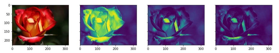

形态转换 (Morphological Transformations)

The term morphological transformation refers to any modification involving the shape and form of the images. These are very often used in image analysis tasks. Although they are used with all types of images, they are especially powerful for images that are not natural (come from a source other than a picture of the real world). The typical transformations are erosion, dilation, opening, and closing. Let’s now look at some code to implement these morphological transformations.

术语形态变换是指涉及图像形状和形式的任何修饰。 这些通常在图像分析任务中使用。 尽管它们可用于所有类型的图像，但对于非自然的图像(来自真实世界的图片以外的其他来源)，它们尤其强大。 典型的转换是侵蚀，膨胀，打开和关闭。 现在让我们看一些实现这些形态转换的代码。

1.Thresholding

1.阈值

One of the simpler operations where we take all the pixels whose intensities are above a certain threshold and convert them to ones; the pixels having value less than the threshold are converted to zero. This results in a binary image.

一种比较简单的操作，其中我们将强度高于特定阈值的所有像素都转换为像素； 值小于阈值的像素将转换为零。 这将产生二进制图像 。

# bin_image will be a (240, 320) True/False array#The range of pixel varies between 0 to 255#The pixel having black is more close to 0 and pixel which is white is more close to 255# 125 is Arbitrary heuristic measure halfway between 1 and 255 (the range of image pixel) bin_image = image[:, :, 0] > 125plot_image([image, bin_image], cmap='gray')

2.Erosion, Dilation, Opening & Closing

2.侵蚀，膨胀，开合

Erosion shrinks bright regions and enlarges dark regions. Dilation on the other hand is exact opposite side — it shrinks dark regions and enlarges the bright regions.

侵蚀使明亮的区域收缩，使黑暗的区域扩大。 另一方面， 膨胀恰好在相反的一面-它会缩小深色区域并扩大明亮区域。

Opening is erosion followed by dilation. Opening can remove small bright spots (i.e. “salt”) and connect small dark cracks. This tends to “open” up (dark) gaps between (bright) features.

开放是侵蚀，然后是膨胀。 开口可以去除小的亮点(即“盐”)并连接小的暗裂纹。 这往往会“打开”(亮)特征之间的(暗)间隙。

Closing is dilation followed by erosion. Closing can remove small dark spots (i.e. “pepper”) and connect small bright cracks. This tends to “close” up (dark) gaps between (bright) features.

关闭是扩张，然后是侵蚀。 关闭可以消除小黑点(即“胡椒”)并连接小亮点。 这往往会“缩小”(亮)特征之间的(暗)间隙。

All these can be done using the skimage.morphology module. The basic idea is to have a circular disk of a certain size (3 below) move around the image and apply these transformations using it.

所有这些都可以使用skimage.morphology模块完成。 基本思想是让一定大小(以下为3)的圆盘在图像周围移动并使用该图像应用这些转换。

from skimage.morphology import binary_closing, binary_dilation, binary_erosion, binary_openingfrom skimage.morphology import selem# use a disk of radius 3selem = selem.disk(3)# oprning and closingopen_img = binary_opening(bin_image, selem)close_img = binary_closing(bin_image, selem)# erosion and dilationeroded_img = binary_erosion(bin_image, selem)dilated_img = binary_dilation(bin_image, selem)plot_image([bin_image, open_img, close_img, eroded_img, dilated_img], cmap='gray')

正常化 (Normalisation)

Normalisation is the most crucial step in the pre-processing part. This refers to rescaling the pixel values so that they lie within a confined range. One of the reasons to do this is to help with the issue of propagating gradients. There are multiple ways to normalize images that we will be talking about.

标准化是预处理部分中最关键的步骤。 这是指重新缩放像素值，以使其位于限定范围内。 这样做的原因之一是帮助解决传播梯度的问题。 我们将讨论多种标准化图像的方法。

#way1-this is common technique followed in case of RGB images norm1_image = image/255#way2-in case of medical Images/non natural images norm2_image = image - np.min(image)/np.max(image) - np.min(image)#way3-in case of medical Images/non natural images norm3_image = image - np.percentile(image,5)/ np.percentile(image,95) - np.percentile(image,5)plot_image([image, norm1_image, norm2_image, norm3_image], cmap='gray')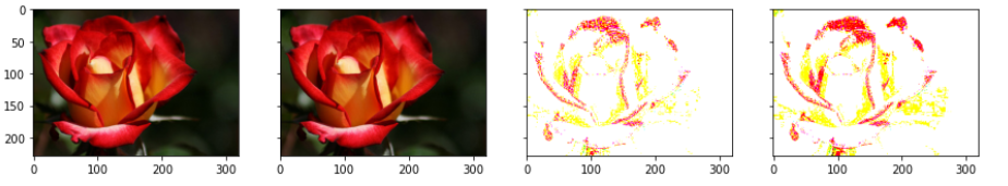

增广 (Augmentation)

This brings us to the next aspect of data pre-processing — data augmentation. Many times, the quantity of data that we have is not sufficient to perform the task of classification well enough. In such cases, we perform data augmentation. As an example, if we are working with a dataset of classifying gemstones into their different types, we may not have enough number of images (since high-quality images are difficult to obtain). In this case, we can perform augmentation to increase the size of your dataset. Augmentation is often used in image-based deep learning tasks to increase the amount and variance of training data. Augmentation should only be done on the training set, never on the validation set.

这使我们进入了数据预处理的下一个方面-数据增强。 很多时候， 我们拥有的数据量不足以充分执行分类任务。 在这种情况下，我们将执行数据扩充 。 例如，如果我们正在使用将宝石分类为不同类型的数据集，则可能没有足够数量的图像(因为很难获得高质量的图像)。 在这种情况下，我们可以执行扩充以增加数据集的大小。 增强通常用于基于图像的深度学习任务中，以增加训练数据的数量和方差。 增强只能在训练集上进行，而不能在验证集上进行。

As you know that pooling increases the invariance. If a picture of a dog is in the top left corner of an image, with pooling, you would be able to recognize if the dog is in little bit left/right/up/down around the top left corner. But with training data consisting of data augmentation like flipping, rotation, cropping, translation, illumination, scaling, adding noise, etc., the model learns all these variations. This significantly boosts the accuracy of the model. So, even if the dog is there at any corner of the image, the model will be able to recognize it with high accuracy.

如您所知， 合并会增加不变性。 如果狗的图片位于图像的左上角，则通过合并，您将能够识别出狗是否在左上角的左/右/上/下一点点。 但是，通过包含翻转，旋转，裁剪，平移，照度，缩放，添加噪声等数据增强的训练数据，该模型可以学习所有这些变化。 这大大提高了模型的准确性。 因此，即使狗在图像的任何角落，模型也将能够高精度地识别它。

There are multiple types of augmentations possible. The basic ones transform the original image using one of the following types of transformations:

可能有多种类型的扩充。 基本的使用以下类型的转换之一来转换原始图像：

1. Linear transformations线性变换
2. Affine transformations仿射变换

from skimage import transform as tf# flip left-right, up-downimage_flipr = np.fliplr(image)image_flipud = np.flipud(image)plot_image([image, image_flipr, image_flipud])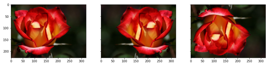

# specify x and y coordinates to be used for shifting (mid points)shift_x, shift_y = image.shape[0]/2, image.shape[1]/2# translation by certain unitsmatrix_to_topleft = tf.SimilarityTransform(translation=[-shift_x, -shift_y])matrix_to_center = tf.SimilarityTransform(translation=[shift_x, shift_y])# rotationrot_transforms =  tf.AffineTransform(rotation=np.deg2rad(45))rot_matrix = matrix_to_topleft + rot_transforms + matrix_to_centerrot_image = tf.warp(image, rot_matrix)# scaling scale_transforms = tf.AffineTransform(scale=(2, 2))scale_matrix = matrix_to_topleft + scale_transforms + matrix_to_centerscale_image_zoom_out = tf.warp(image, scale_matrix)scale_transforms = tf.AffineTransform(scale=(0.5, 0.5))scale_matrix = matrix_to_topleft + scale_transforms + matrix_to_centerscale_image_zoom_in = tf.warp(image, scale_matrix)# translationtransaltion_transforms = tf.AffineTransform(translation=(50, 50))translated_image = tf.warp(image, transaltion_transforms)plot_image([image, rot_image, scale_image_zoom_out, scale_image_zoom_in, translated_image])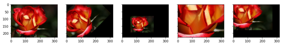

# shear transformsshear_transforms = tf.AffineTransform(shear=np.deg2rad(45))shear_matrix = matrix_to_topleft + shear_transforms + matrix_to_centershear_image = tf.warp(image, shear_matrix)bright_jitter = image*0.999 + np.zeros_like(image)*0.001plot_image([image, shear_image, bright_jitter])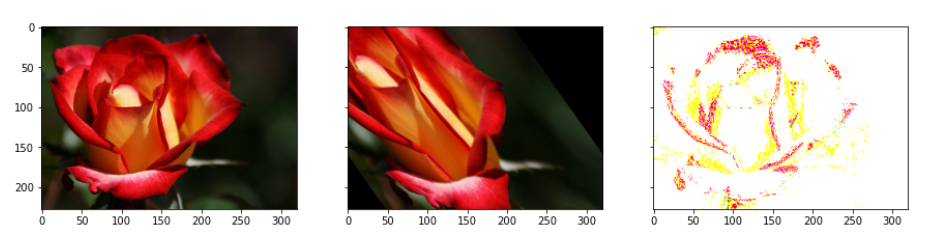

网络建设 (Network Building)

Let’s now build and train the model.

现在让我们构建和训练模型。

选择架构 (Choosing the architecture)

We will use ‘ResNet’ architecture in this section. Since ResNets have become quite prevalent in the industry, it is worth spending some time to understand the important elements of their architecture. Let’s start with the original architecture proposed here. Also, in 2016, the ResNet team had proposed some improvements in the original architecture here. Using these modifications, they had trained nets of more than 1000 layers (e.g. ResNet-1001).

在本节中，我们将使用“ ResNet ”架构。 由于ResNets在行业中已变得相当普遍，因此值得花一些时间来了解其体系结构的重要元素。 让我们从这里提出的原始架构开始 。 此外，在2016年，RESNET队曾提议在原有的架构有所改善这里 。 使用这些修改，他们训练了超过1000层的网络 (例如ResNet-1001 )。

The ‘ResNet builder’ module which is used here is basically a Python module containing all the building blocks of ResNet. We will use this module to import the variants of ResNets (ResNet-18, ResNet-34, etc.). The resnet.py module is taken from here. Its biggest upside is that the ‘skip connections’ mechanism allows very deep networks.

这里使用的“ ResNet builder”模块基本上是一个Python模块，其中包含ResNet的所有构建块。 我们将使用此模块导入ResNet的变体(ResNet-18，ResNet-34等)。 resnet.py模块来自此处 。 其最大的好处是“跳过连接”机制允许非常深的网络。

运行数据生成器 (Run a data generator)

Data generator supports preprocessing — it normalizes the images (dividing by 255) and crops the center (100 x 100) portion of the image.

数据生成器支持预处理-标准化图像(除以255)并裁剪图像的中心(100 x 100)部分。

There was no specific reason to include 100 as the dimension but it has been chosen so that we can process all the images which are of greater than 100*100 dimension. If any dimension (height or width) of an image is less than 100 pixels, then that image is deleted automatically. You can change it to 150 or 200 according to your need.

没有特别的理由将100作为尺寸，但是选择它是为了我们可以处理所有尺寸大于100 * 100的图像。 如果图像的任何尺寸(高度或宽度)小于100像素，则该图像将被自动删除。 您可以根据需要将其更改为150或200。

Let’s now set up the data generator. The code below sets up a custom data generator which is slightly different than the one that comes with the keras API. The reason to use a custom generator is to be able to modify it according to the problem at hand (customizability).

现在设置数据生成器 。 下面的代码设置了一个自定义数据生成器，该数据生成器与keras API附带的自定义数据生成器略有不同。 使用定制生成器的原因是能够根据当前问题(可定制性)对其进行修改。

import numpy as npimport kerasclass DataGenerator(keras.utils.Sequence):    'Generates data for Keras'

    def __init__(self, mode='train', ablation=None, flowers_cls=['daisy', 'rose'],                  batch_size=32, dim=(100, 100), n_channels=3, shuffle=True):        """        Initialise the data generator        """        self.dim = dim        self.batch_size = batch_size        self.labels = {}        self.list_IDs = []

        # glob through directory of each class         for i, cls in enumerate(flowers_cls):            paths = glob.glob(os.path.join(DATASET_PATH, cls, '*'))            brk_point = int(len(paths)*0.8)            if mode == 'train':                paths = paths[:brk_point]            else:                paths = paths[brk_point:]            if ablation is not None:                paths = paths[:ablation]            self.list_IDs += paths            self.labels.update({p:i for p in paths})

        self.n_channels = n_channels        self.n_classes = len(flowers_cls)        self.shuffle = shuffle        self.on_epoch_end()    def __len__(self):        'Denotes the number of batches per epoch'        return int(np.floor(len(self.list_IDs) / self.batch_size))    def __getitem__(self, index):        'Generate one batch of data'        # Generate indexes of the batch        indexes = self.indexes[index*self.batch_size:(index+1)*self.batch_size]        # Find list of IDs        list_IDs_temp = [self.list_IDs[k] for k in indexes]        # Generate data        X, y = self.__data_generation(list_IDs_temp)        return X, y    def on_epoch_end(self):        'Updates indexes after each epoch'        self.indexes = np.arange(len(self.list_IDs))        if self.shuffle == True:            np.random.shuffle(self.indexes)    def __data_generation(self, list_IDs_temp):        'Generates data containing batch_size samples' # X : (n_samples, *dim, n_channels)        # Initialization        X = np.empty((self.batch_size, *self.dim, self.n_channels))        y = np.empty((self.batch_size), dtype=int)

        delete_rows = []        # Generate data        for i, ID in enumerate(list_IDs_temp):            # Store sample            img = io.imread(ID)            img = img/255            if img.shape[0] > 100 and img.shape[1] > 100:                h, w, _ = img.shape                img = img[int(h/2)-50:int(h/2)+50, int(w/2)-50:int(w/2)+50, : ]            else:                delete_rows.append(i)                continue

            X[i,] = img

            # Store class            y[i] = self.labels[ID]

        X = np.delete(X, delete_rows, axis=0)        y = np.delete(y, delete_rows, axis=0)        return X, keras.utils.to_categorical(y, num_classes=self.n_classes)

To start with, we have the training data stored in nn directories (if there are nn classes). For a given batch size, we want to generate batches of data points and feed them to the model.

首先，我们将训练数据存储在nn目录中(如果有nn个类)。 对于给定的批处理大小，我们希望生成一批数据点并将其馈送到模型中。

The first for loop 'globs' through each of the classes (directories). For each class, it stores the path of each image in the list paths. In training mode, it subsets paths to contain the first 80% images; in validation mode it subsets the last 20%. In the special case of an ablation experiment, it simply subsets the first ablation images of each class.

每个类(目录)的第一个for循环“全局对象”。 对于每个类，它将每个图像的路径存储在列表paths 。 在训练模式下，它对paths进行子集以包含前80％的图像； 在验证模式下，它会将最后20％的内容作为子集。 在消融实验的特殊情况下，它只是将每个类别的第一个ablation图像进行子集化。

We store the paths of all the images (of all classes) in a combined list self.list_IDs. The dictionary self.labels contains the labels (as key:value pairs of path: class_number (0/1)).

我们将所有图像(所有类)的路径存储在组合列表self.list_IDs 。 字典self.labels包含标签(作为path: class_number (0/1) key：value对path: class_number (0/1) )。

After the loop, we call the method on_epoch_end(), which creates an array self.indexes of length self.list_IDs and shuffles them (to shuffle all the data points at the end of each epoch).

循环之后，我们调用方法on_epoch_end() ，该方法创建一个长度为self.list_IDs的数组self.list_IDs并self.indexes进行self.list_IDs (以在每个纪元末尾对所有数据点进行self.list_IDs )。

The _getitem_ method uses the (shuffled) array self.indexes to select a batch_size number of entries (paths) from the path list self.list_IDs.

该_getitem_方法使用(洗牌)阵列self.indexes选择batch_size从路径列表中的条目(路径)数self.list_IDs 。

Finally, the method __data_generation returns the batch of images as the pair X, y where X is of shape (batch_size, height, width, channels) and y is of shape (batch size, ). Note that __data_generation also does some preprocessing - it normalises the images (divides by 255) and crops the center 100 x 100 portion of the image. Thus, each image has the shape (100, 100, num_channels). If any dimension (height or width) of an image less than 100 pixels, that image is deleted.

最后，方法__data_generation返回成对的图像批次X，y，其中X的形状为(batch_size, height, width, channels)而y的形状为(batch size, ) 。 请注意， __data_generation还执行一些预处理-将图像__data_generation (除以255)并__data_generation图像中心100 x 100。 因此，每个图像具有形状(100, 100, num_channels) 。 如果图像的任何尺寸(高度或宽度)小于100像素，则会删除该图像。

消融实验 (Ablation Experiments)

These refer to taking a small chunk of data and running your model on it — this helps in figuring out if the model is running at all. This is called an ablation experiment.

这些指的是获取一小部分数据并在其上运行模型-这有助于确定模型是否在运行。 这称为消融实验。

The first part of building a network is to get it to run on your dataset. Let’s try fitting the net on only a few images and just one epoch. Note that since ablation=100 is specified, 100 images of each class are used, so total number of batches is np.floor(200/32) = 6.

构建网络的第一步是使它在数据集上运行。 让我们尝试仅在少数几个图像和一个纪元上拟合网络。 请注意，由于指定了ablation=100 ，因此每个类别使用100张图像，因此批次总数为np.floor(200/32) = 6。

Note that the DataGenerator class 'inherits' from the keras.utils.Sequence class, so it has all the functionalities of the base keras.utils.Sequence class (such as the model.fit_generator method).

注意， DataGenerator从类继承“ keras.utils.Sequence类，因此它具有基的所有功能keras.utils.Sequence类(如model.fit_generator方法)。

# using resnet 18model = resnet.ResnetBuilder.build_resnet_18((img_channels, img_rows, img_cols), nb_classes)model.compile(loss='categorical_crossentropy', optimizer='SGD',              metrics=['accuracy'])# create data generator objects in train and val mode# specify ablation=number of data points to train ontraining_generator = DataGenerator('train', ablation=100)validation_generator = DataGenerator('val', ablation=100)# fit: this will fit the net on 'ablation' samples, only 1 epochmodel.fit_generator(generator=training_generator,                    validation_data=validation_generator,                    epochs=1,)

过度拟合训练数据 (Overfitting on Training Data)

The next step is trying to overfit the model on the training data. Why would we want to intentionally overfit on our data? Simply put, this will tell us whether the network is capable of learning the patterns in the training set. This tells you whether the model is behaving as expected or not.

下一步是尝试对训练数据过度拟合模型。 我们为什么要故意过度拟合我们的数据？ 简而言之，这将告诉我们网络是否能够学习训练集中的模式。 这将告诉您模型是否表现出预期的行为。

We’ll use ablation=100 (i.e. training on 100 images of each class), so it is still a very small dataset, and we will use 20 epochs. In each epoch, 200/32=6 batches will be used.

我们将使用ablation = 100(即在每个类上训练100张图像)，因此它仍然是一个非常小的数据集，并且将使用20个纪元。 在每个时代，将使用200/32 = 6批。

# resnet 18model = resnet.ResnetBuilder.build_resnet_18((img_channels, img_rows, img_cols), nb_classes)model.compile(loss='categorical_crossentropy',optimizer='SGD',              metrics=['accuracy'])# generatorstraining_generator = DataGenerator('train', ablation=100)validation_generator = DataGenerator('val', ablation=100)# fitmodel.fit_generator(generator=training_generator,                    validation_data=validation_generator,                    epochs=20)

The results show that the training accuracy increases consistently with each epoch. The validation accuracy also increases and then plateaus out — this is a sign of ‘good fit’, i.e. we know that the model is at least able to learn from a small dataset, so we can hope that it will be able to learn from the entire set as well.

结果表明，训练精度随着每个时期的增加而一致。 验证准确性也会提高，然后达到平稳状态–这是“良好拟合”的标志，即我们知道该模型至少能够从较小的数据集中学习，因此我们希望它能够从整套也是如此。

To summarise, a good test of any model is to check whether it can overfit on the training data (i.e. the training loss consistently reduces along epochs). This technique is especially useful in deep learning because most deep learning models are trained on large datasets, and if they are unable to overfit a small version, then they are unlikely to learn from the larger version.

综上所述，对任何模型的一个很好的测试是检查它是否可以对训练数据过度拟合 (即训练损失沿历时不断减少)。 这项技术在深度学习中特别有用，因为大多数深度学习模型都是在大型数据集上进行训练的，并且如果它们无法适合较小的版本，则他们不太可能从较大的版本中学习。

超参数调整 (Hyperparameter tuning)

we trained the model on a small chunk of the dataset and confirmed that the model can learn from the dataset (indicated by overfitting). After fixing the model and data augmentation, we now need to find the learning rate for the optimizer (here SGD). First, let’s make a list of the hyper-parameters we want to tune:

我们在数据集中的一小部分上对模型进行了训练，并确认该模型可以从数据集中学习(通过过度拟合表示)。 修正模型和数据扩充之后，我们现在需要找到优化器的学习率(此处为SGD)。 首先，让我们列出要调整的超参数：

1. Learning Rate & Variation + Optimisers学习率与变异+优化器
2. Augmentation Techniques增强技术

The basic idea is to track the validation loss with increasing epochs for various values of a hyperparameter.

基本思想是随着超参数的各种值的增加而跟踪验证损失。

Keras Callbacks

Keras回调

Before you move ahead, let’s discuss a bit about callbacks. Callbacks are basically actions that you want to perform at specific instances of training. For example, we want to perform the action of storing the loss at the end of every epoch (the instance here is the end of an epoch).

在继续之前，让我们讨论一下回调 。 回调基本上是您想要在特定训练实例上执行的操作。 例如，我们想要执行在每个时期结束时存储损失的操作(这里的实例是一个时期的结束)。

Formally, a callback is simply a function (if you want to perform a single action), or a list of functions (if you want to perform multiple actions), which are to be executed at specific events (end of an epoch, start of every batch, when the accuracy plateaus out, etc.). Keras provides some very useful callback functionalities through the class keras.callbacks.Callback.

形式上，回调只是一个函数(如果要执行单个动作)或函数列表(如果要执行多个动作)，它们将在特定事件(时期结束，开始时)执行每批，精度达到稳定水平时等)。 keras.callbacks.Callback通过类keras.callbacks.Callback提供了一些非常有用的回调功能。

Keras has many builtin callbacks (listed here). The generic way to create a custom callback in keras is:

Keras有许多内置的回调( 在此处列出 )。 在keras中创建自定义回调的通用方法是：

from keras import optimizersfrom keras.callbacks import *# range of learning rates to tunehyper_parameters_for_lr = [0.1, 0.01, 0.001]# callback to append lossclass LossHistory(keras.callbacks.Callback):    def on_train_begin(self, logs={}):        self.losses = []    def on_epoch_end(self, epoch, logs={}):        self.losses.append(logs.get('loss'))# instantiate a LossHistory() object to store historieshistory = LossHistory()plot_data = {}# for each hyperparam: train the model and plot loss historyfor lr in hyper_parameters_for_lr:    print ('\n\n'+'=='*20 + '   Checking for LR={}  '.format(lr) + '=='*20 )    sgd = optimizers.SGD(lr=lr, clipnorm=1.)        # model and generators    model = resnet.ResnetBuilder.build_resnet_18((img_channels, img_rows, img_cols), nb_classes)    model.compile(loss='categorical_crossentropy',optimizer= sgd,                  metrics=['accuracy'])    training_generator = DataGenerator('train', ablation=100)    validation_generator = DataGenerator('val', ablation=100)    model.fit_generator(generator=training_generator,                        validation_data=validation_generator,                        epochs=3, callbacks=[history])        # plot loss history    plot_data[lr] = history.losses

In the code above, we have created a custom callback to append the loss to a list at the end of every epoch. Note that logs is an attribute (a dictionary) of keras.callbacks.Callback, and we are using it to get the value of the key 'loss'. Some other keys of this dict are acc, val_loss etc.

在上面的代码中，我们创建了一个自定义回调，以将损失附加到每个时期末尾的列表中。 请注意， logs是keras.callbacks.Callback的属性(字典)，我们正在使用它来获取键“ loss”的值。 此字典的其他一些键是acc ， val_loss等。

To tell the model that we want to use a callback, we create an object of LossHistory called history and pass it to model.fit_generator using callbacks=[history]. In this case, we only have one callback history, though you can pass multiple callback objects through this list (an example of multiple callbacks is in the section below - see the code block of DecayLR()).

为了告诉模型我们要使用回调，我们创建了一个名为history的LossHistory对象，并使用callbacks=[history]将其传递给model.fit_generator 。 在这种情况下，我们只有一个回调history ，尽管您可以通过此列表传​​递多个回调对象(以下部分中为多个回调的示例-请参见DecayLR()的代码块)。

Here, we tuned the learning rate hyperparameter and observed that a rate of 0.1 is the optimal learning rate when compared to 0.01 and 0.001. However, using such a high learning rate for the entire training process is not a good idea since the loss may start to oscillate around the minima later. So, at the start of the training, we use a high learning rate for the model to learn fast, but as we train further and proceed towards the minima, we decrease the learning rate gradually.

在这里， 我们调整了学习率超参数，并观察到与0.01和0.001相比，0.1是最佳学习率。 但是，在整个训练过程中使用如此高的学习率并不是一个好主意，因为稍后损失可能会开始围绕最小值移动。 因此，在训练开始时，我们使用较高的学习率来使模型快速学习，但是随着我们进一步训练并朝着最小值迈进，我们会逐渐降低学习率。

# plot loss history for each value of hyperparameterf, axes = plt.subplots(1, 3, sharey=True)f.set_figwidth(15)plt.setp(axes, xticks=np.arange(0, len(plot_data[0.01]), 1)+1)for i, lr in enumerate(plot_data.keys()):    axes[i].plot(np.arange(len(plot_data[lr]))+1, plot_data[lr])

The results above show that a learning rate of 0.1 is the best, though using such a high learning rate for the entire training is usually not a good idea. Thus, we should use learning rate decay — starting from a high learning rate and decaying it with every epoch.

上面的结果表明，学习速度最好为0.1，尽管在整个训练过程中使用如此高的学习速度通常不是一个好主意。 因此，我们应该使用学习率衰减 -从较高的学习率开始，然后在每个时期都将其衰减。

We use another custom callback (DecayLR) to decay the learning rate at the end of every epoch. The decay rate is specified as 0.5 ^ epoch. Also, note that this time we are telling the model to use two callbacks (passed as a list callbacks=[history, decay] to model.fit_generator).

我们使用另一个自定义回调 ( DecayLR )在每个时期结束时降低学习率。 衰减率指定为0.5 ^ epoch。 另外，请注意，这次我们告诉模型使用两个回调 (作为列表callbacks=[history, decay]传递给model.fit_generator callbacks=[history, decay] )。

Although we have used our own custom decay implementation here, you can use the ones built into keras optimisers (using the decay argument).

尽管我们在这里使用了自己的自定义衰减实现，但是您可以使用内置在keras优化器中的实现 (使用decay参数)。

# learning rate decayclass DecayLR(keras.callbacks.Callback):    def __init__(self, base_lr=0.001, decay_epoch=1):        super(DecayLR, self).__init__()        self.base_lr = base_lr        self.decay_epoch = decay_epoch         self.lr_history = []

    # set lr on_train_begin    def on_train_begin(self, logs={}):        K.set_value(self.model.optimizer.lr, self.base_lr)    # change learning rate at the end of epoch    def on_epoch_end(self, epoch, logs={}):        new_lr = self.base_lr * (0.5 ** (epoch // self.decay_epoch))        self.lr_history.append(K.get_value(self.model.optimizer.lr))        K.set_value(self.model.optimizer.lr, new_lr)# to store loss historyhistory = LossHistory()plot_data = {}# start with lr=0.1decay = DecayLR(base_lr=0.1)# modelsgd = optimizers.SGD()model = resnet.ResnetBuilder.build_resnet_18((img_channels, img_rows, img_cols), nb_classes)model.compile(loss='categorical_crossentropy',optimizer= sgd,              metrics=['accuracy'])training_generator = DataGenerator('train', ablation=100)validation_generator = DataGenerator('val', ablation=100)model.fit_generator(generator=training_generator,                    validation_data=validation_generator,                    epochs=3, callbacks=[history, decay])plot_data[lr] = decay.lr_history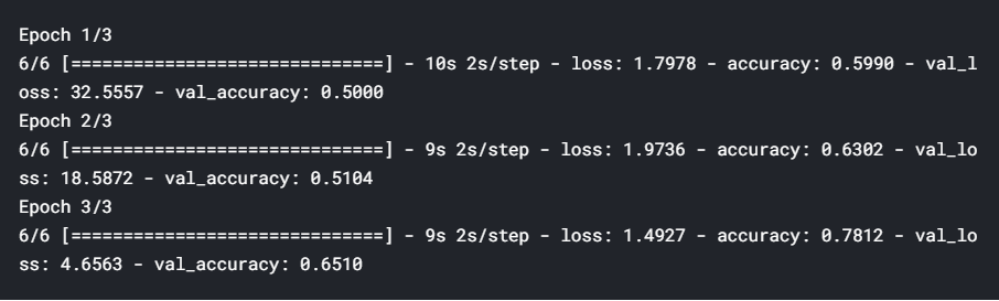

plt.plot(np.arange(len(decay.lr_history)), decay.lr_history)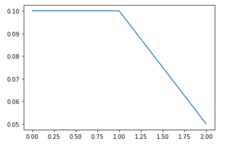

Augmentation Techniques

增强技术

Let’s now write some code to implement data augmentation. Augmentation is usually done with data generators, i.e. the augmented data is generated batch-wise, on the fly. You can either use the built-in keras ImageDataGenerator or write your own data generator (for some custom features etc if you want). The below code show how to implement these.

现在让我们编写一些代码来实现数据扩充。 增强通常是通过数据生成器完成的，即增强的数据是动态地分批生成的。 您可以使用内置的keras ImageDataGenerator或编写自己的数据生成器(如果需要，可以使用某些自定义功能等)。 下面的代码显示了如何实现这些。

import numpy as npimport keras# data generator with augmentationclass AugmentedDataGenerator(keras.utils.Sequence):    'Generates data for Keras'    def __init__(self, mode='train', ablation=None, flowers_cls=['daisy', 'rose'],                  batch_size=32, dim=(100, 100), n_channels=3, shuffle=True):        'Initialization'        self.dim = dim        self.batch_size = batch_size        self.labels = {}        self.list_IDs = []        self.mode = mode

        for i, cls in enumerate(flowers_cls):            paths = glob.glob(os.path.join(DATASET_PATH, cls, '*'))            brk_point = int(len(paths)*0.8)            if self.mode == 'train':                paths = paths[:brk_point]            else:                paths = paths[brk_point:]            if ablation is not None:                paths = paths[:ablation]            self.list_IDs += paths            self.labels.update({p:i for p in paths})

        self.n_channels = n_channels        self.n_classes = len(flowers_cls)        self.shuffle = shuffle        self.on_epoch_end()    def __len__(self):        'Denotes the number of batches per epoch'        return int(np.floor(len(self.list_IDs) / self.batch_size))    def __getitem__(self, index):        'Generate one batch of data'        # Generate indexes of the batch        indexes = self.indexes[index*self.batch_size:(index+1)*self.batch_size]        # Find list of IDs        list_IDs_temp = [self.list_IDs[k] for k in indexes]        # Generate data        X, y = self.__data_generation(list_IDs_temp)        return X, y    def on_epoch_end(self):        'Updates indexes after each epoch'        self.indexes = np.arange(len(self.list_IDs))        if self.shuffle == True:            np.random.shuffle(self.indexes)    def __data_generation(self, list_IDs_temp):        'Generates data containing batch_size samples' # X : (n_samples, *dim, n_channels)        # Initialization        X = np.empty((self.batch_size, *self.dim, self.n_channels))        y = np.empty((self.batch_size), dtype=int)

        delete_rows = []        # Generate data        for i, ID in enumerate(list_IDs_temp):            # Store sample            img = io.imread(ID)            img = img/255            if img.shape[0] > 100 and img.shape[1] > 100:                h, w, _ = img.shape                img = img[int(h/2)-50:int(h/2)+50, int(w/2)-50:int(w/2)+50, : ]            else:                delete_rows.append(i)                continue

            X[i,] = img

            # Store class            y[i] = self.labels[ID]

        X = np.delete(X, delete_rows, axis=0)        y = np.delete(y, delete_rows, axis=0)                # data augmentation        if self.mode == 'train':            aug_x = np.stack([datagen.random_transform(img) for img in X])            X = np.concatenate([X, aug_x])            y = np.concatenate([y, y])        return X, keras.utils.to_categorical(y, num_classes=self.n_classes)

Metrics to optimize

优化指标

Depending on the situation, we choose the appropriate metrics. For binary classification problems, AUC is usually the best metric.

根据情况，我们选择适当的指标。 对于二进制分类问题，AUC通常是最佳度量。

AUC is often a better metric than accuracy. So instead of optimising for accuracy, let’s monitor AUC and choose the best model based on AUC on validation data. We’ll use the callbacks on_train_begin and on_epoch_end to initialize (at the start of each epoch) and store the AUC (at the end of epoch).

AUC通常比准确度更好。 因此，让我们监控AUC并根据验证数据选择基于AUC的最佳模型，而不是针对准确性进行优化。 我们将使用回调on_train_begin和on_epoch_end进行初始化(在每个纪元的开始)并存储AUC(在纪元的末尾)。

from sklearn.metrics import roc_auc_scoreclass roc_callback(Callback):

    def on_train_begin(self, logs={}):        logs['val_auc'] = 0    def on_epoch_end(self, epoch, logs={}):        y_p = []        y_v = []        for i in range(len(validation_generator)):            x_val, y_val = validation_generator[i]            y_pred = self.model.predict(x_val)            y_p.append(y_pred)            y_v.append(y_val)        y_p = np.concatenate(y_p)        y_v = np.concatenate(y_v)        roc_auc = roc_auc_score(y_v, y_p)        print ('\nVal AUC for epoch{}: {}'.format(epoch, roc_auc))        logs['val_auc'] = roc_auc

决赛 (Final Run)

Let’s now train the final model. Note that we will keep saving the best model’s weights at models/best_models.hdf5, so you will need to create a directory models. Note that model weights are usually saved in hdf5 files.

现在让我们训练最终模型。 请注意，我们将继续将最佳模型的权重保存在models/best_models.hdf5 ，因此您将需要创建目录models 。 请注意，模型权重通常保存在hdf5文件中。

Saving the best model is done using the callback functionality that comes with ModelCheckpoint. We basically specify the filepath where the model weights are to be saved, monitor='val_auc' specifies that you are choosing the best model based on validation accuracy, save_best_only=True saves only the best weights, and mode='max' specifies that the validation accuracy is to be maximized.

使用ModelCheckpoint随附的回调功能可以保存最佳模型 。 我们基本上指定了要保存模型权重的文件filepath ， monitor='val_auc'指定您要根据验证准确性选择最佳模型， save_best_only=True仅保存最佳权重，而mode='max'指定验证准确性应最大化。

# modelmodel = resnet.ResnetBuilder.build_resnet_18((img_channels, img_rows, img_cols), nb_classes)model.compile(loss='categorical_crossentropy',optimizer= sgd,              metrics=['accuracy'])training_generator = AugmentedDataGenerator('train', ablation=32)validation_generator = AugmentedDataGenerator('val', ablation=32)# checkpoint filepath = 'models/best_model.hdf5'checkpoint = ModelCheckpoint(filepath, monitor='val_auc', verbose=1, save_best_only=True, mode='max')auc_logger = roc_callback()# fit model.fit_generator(generator=training_generator,                    validation_data=validation_generator,                    epochs=3, callbacks=[auc_logger, history, decay, checkpoint])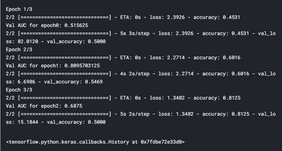

plt.imshow(image)

#standardizing image#moved the origin to the centre of the imageh, w, _ = image.shapeimg = image[int(h/2)-50:int(h/2)+50, int(w/2)-50:int(w/2)+50, : ]model.predict(img[np.newaxis,: ])

Hey, we have got a very high probability for class 1 i.e. rose. If you remember, class 0 was daisy and class 1 was rose(on top of the blog). So, the model has learnt perfectly. We have built a model with a good AUC at the end of 3 epochs. If you train this using more epochs, you should be able to reach a better AUC value.

嘿，我们有很高的可能性上1类，即上升。 如果您还记得的话，班级0是雏菊，班级1是玫瑰(在博客顶部)。 因此，该模型学得很完美。 我们已经建立了一个模型，该模型在3个阶段结束时具有良好的AUC。 如果您使用更多的时间进行训练，则应该能够达到更好的AUC值。

If you have any questions, recommendations or critiques, I can be reached via LinkedIn or the comment section.

如果您有任何疑问，建议或批评，请通过LinkedIn或评论栏与我联系。