介绍 (Introduction)

Decision Trees (DTs) are a non-parametric supervised learning method used for classification and regression. The goal is to create a model that predicts the value of a target variable by learning simple decision rules inferred from the data features. Decision trees are commonly used in operations research, specifically in decision analysis, to help identify a strategy most likely to reach a goal, but are also a popular tool in machine learning.

决策树(DT)是一种用于分类和回归的非参数监督学习方法。 目标是创建一个模型，该模型通过学习从数据特征推断出的简单决策规则来预测目标变量的值。 决策树通常用于运营研究中，尤其是决策分析中，用于帮助确定最有可能达成目标的策略，但它也是机器学习中的一种流行工具。

语境 (Context)

In this article, we will be discussing the following topics

在本文中，我们将讨论以下主题

1. What are decision trees in general一般而言，决策树是什么
2. Types of decision trees.决策树的类型。
3. Algorithms used to build decision trees.用于构建决策树的算法。
4. The step-by-step process of building a Decision tree.建立决策树的分步过程。

什么是决策树？ (What are Decision trees?)

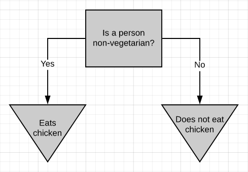
The above picture is a simple decision tree. If a person is non-vegetarian, then he/she eats chicken (most probably), otherwise, he/she doesn’t eat chicken. The decision tree, in general, asks a question and classifies the person based on the answer. This decision tree is based on a yes/no question. It is just as simple to build a decision tree on numeric data.

上图是一个简单的决策树。 如果一个人不是素食者，那么他(她)很可能会吃鸡肉，否则，他/她不会吃鸡肉。 通常，决策树会提出问题并根据答案对人员进行分类。 该决策树基于是/否问题。 在数字数据上构建决策树非常简单。

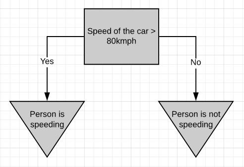
If a person is driving above 80kmph, we can consider it as over-speeding, else not.

如果一个人以每小时80英里的速度行驶，我们可以认为它是超速行驶，否则就不行。

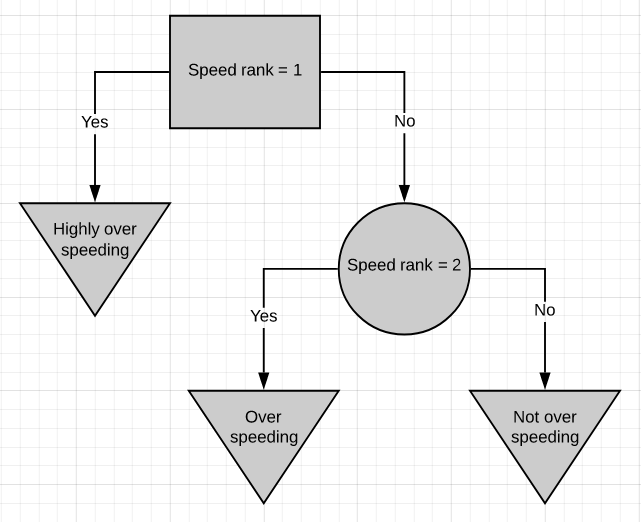
Here is one more simple decision tree. This decision tree is based on ranked data, where 1 means the speed is too high, 2 corresponds to a much lesser speed. If a person is speeding above rank 1 then he/she is highly over-speeding. If the person is above speed rank 2 but below speed rank 1 then he/she is over-speeding but not that much. If the person is below speed rank 2 then he/she is driving well within speed limits.

这是另一种简单的决策树。 该决策树基于排名数据，其中1表示速度太高，2表示速度要低得多。 如果一个人超速超过等级1，那么他/她就极度超速。 如果此人在速度等级2以上但在速度等级1以下，则他/她超速，但不是那么多。 如果该人低于速度等级2，则他/她在速度限制内驾驶得很好。

The classification in a decision tree can be both categoric or numeric.

决策树中的分类可以是分类的，也可以是数字的。

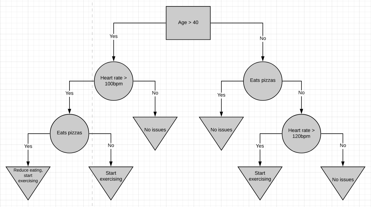
Here’s a more complicated decision tree. It combines numeric data with yes/no data. For the most part Decision trees are pretty simple to work with. You start at the top and work your way down till you get to a point where you cant go further. That’s how a sample is classified.

这是一个更复杂的决策树。 它将数字数据与是/否数据组合在一起。 在大多数情况下，决策树非常简单。 您从顶部开始，一直往下走，直到到达无法继续前进的地步。 这就是样本分类的方式。

The very top of the tree is called the root node or just the root. The nodes in between are called internal nodes. Internal nodes have arrows pointing to them and arrows pointing away from them. The end nodes are called the leaf nodes or just leaves. Leaf nodes have arrows pointing to them but no arrows pointing away from them.

树的最顶端称为根节点 或只是根。 中间的节点称为内部节点 。 内部节点具有指向它们的箭头和指向远离它们的箭头。 末端节点称为叶子节点或仅称为叶子 。 叶节点有指向它们的箭头，但没有指向远离它们的箭头。

In the above diagrams, root nodes are represented by rectangles, internal nodes by circles, and leaf nodes by inverted-triangles.

在上图中，根节点用矩形表示，内部节点用圆形表示，叶节点用倒三角形表示。

建立决策树 (Building a Decision tree)

There are several algorithms to build a decision tree.

有几种算法可以构建决策树。

1. CART-Classification and Regression TreesCART分类和回归树
2. ID3-Iterative Dichotomiser 3ID3迭代二分频器3
3. C4.5C4.5
4. CHAID-Chi-squared Automatic Interaction DetectionCHAID卡方自动交互检测

We will be discussing only CART and ID3 algorithms as they are the ones majorly used.

我们将仅讨论CART和ID3算法，因为它们是最常用的算法。

大车 (CART)

CART is a DT algorithm that produces binary Classification or Regression Trees, depending on whether the dependent (or target) variable is categorical or numeric, respectively. It handles data in its raw form (no preprocessing needed) and can use the same variables more than once in different parts of the same DT, which may uncover complex interdependencies between sets of variables.

CART是一种DT算法，它分别根据因变量(或目标变量)是分类变量还是数字变量而生成二进制 分类树或回归树。 它以原始格式处理数据(无需预处理)，并且可以在同一DT的不同部分中多次使用相同的变量，这可能揭示变量集之间的复杂相互依赖性。

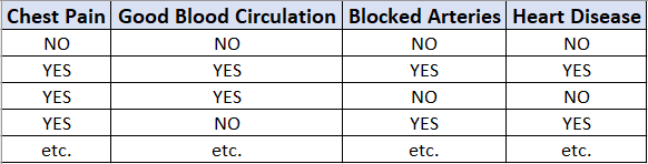
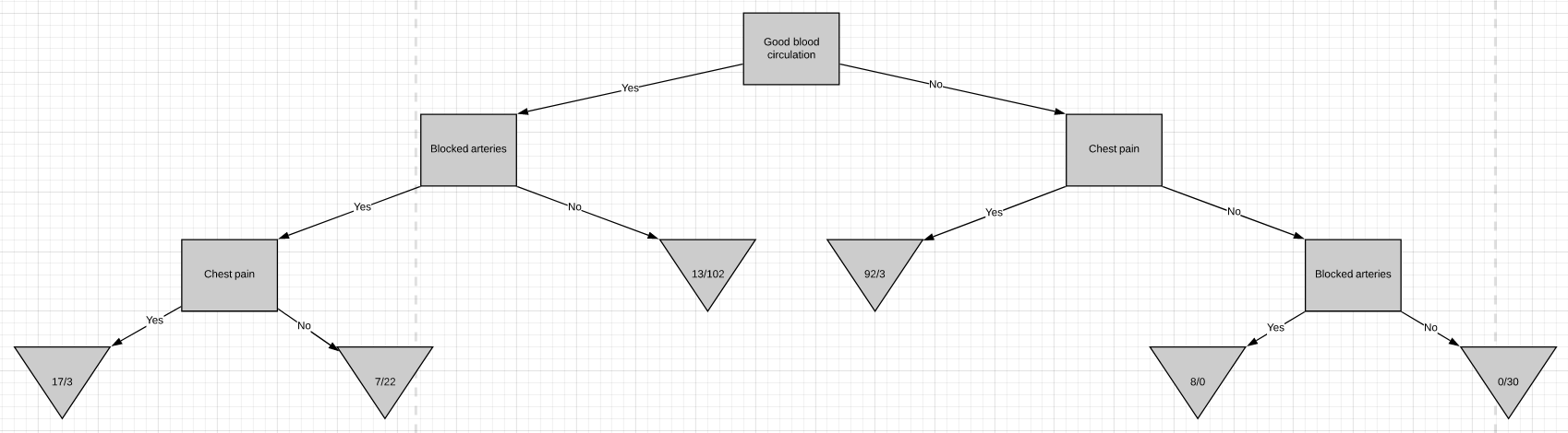
Now we are going to discuss how to build a decision tree from a raw table of data. In the example given above, we will be building a decision tree that uses chest pain, good blood circulation, and the status of blocked arteries to predict if a person has heart disease or not.

现在，我们将讨论如何从原始数据表构建决策树。 在上面给出的示例中，我们将构建一个决策树，该决策树使用胸痛，良好的血液循环以及动脉阻塞的状态来预测一个人是否患有心脏病。

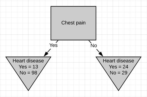
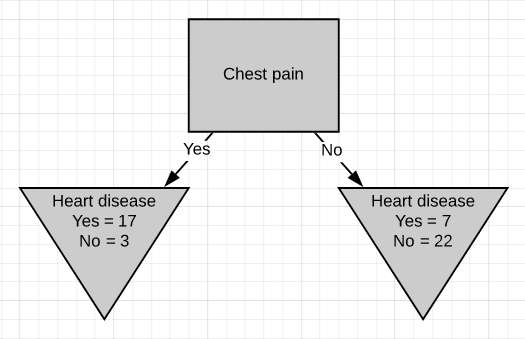
The first thing we have to know is which feature should be on the top or in the root node of the tree. We start by looking at how chest pain alone predicts heart disease.

我们首先要知道的是哪个功能应该在树的顶部或根节点中。 我们首先来看仅胸痛是如何预示心脏病的。

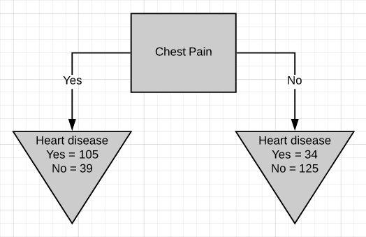
There are two leaf nodes, one each for the two outcomes of chest pain. Each of the leaves contains the no. of patients having heart disease and not having heart disease for the corresponding entry of chest pain. Now we do the same thing for good blood circulation and blocked arteries.

有两个叶结，每个胸结分别导致两种胸痛。 每片叶子都包含no。 患有心脏病而没有心脏病的患者中，有相应的胸痛会进入。 现在，我们为血液循环良好和动脉阻塞做了同样的事情。

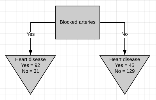
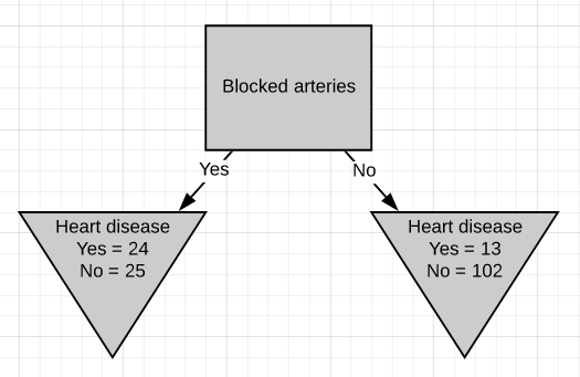
We can see that neither of the 3 features separates the patients having heart disease from the patients not having heart disease perfectly. It is to be noted that the total no. of patients having heart disease is different in all three cases. This is done to simulate the missing values present in real-world datasets.

我们可以看到，这三个特征都没有将患有心脏病的患者与没有患有心脏病的患者完美地分开。 要注意的是总数。 在这三种情况下，患有心脏病的患者的比例均不同。 这样做是为了模拟现实数据集中存在的缺失值。

Because none of the leaf nodes is either 100% ‘yes heart disease’ or 100% ‘no heart disease’, they are all considered impure. To decide on which separation is the best, we need a method to measure and compare impurity.

因为所有叶节点都不是100％“是心脏病”或100％“没有心脏病”，所以它们都被认为是不纯的。 为了确定哪种分离最好，我们需要一种测量和比较杂质的方法。

The metric used in the CART algorithm to measure impurity is the Gini impurity score. Calculating Gini impurity is very easy. Let’s start by calculating the Gini impurity for chest pain.

CART算法中用于测量杂质的度量标准是基尼杂质评分 。 计算基尼杂质非常简单。 让我们从计算吉尼杂质引起的胸痛开始。

For the left leaf,

对于左叶

Gini impurity = 1 - (probability of ‘yes’)² - (probability of ‘no’)²              = 1 - (105/105+39)² - (39/105+39)²Gini impurity = 0.395

Similarly, calculate the Gini impurity for the right leaf node.

同样，计算右叶节点的基尼杂质。

Gini impurity = 1 - (probability of ‘yes’)² - (probability of ‘no’)²              = 1 - (34/34+125)² - (125/34+125)²Gini impurity = 0.336

Now that we have measured the Gini impurity for both leaf nodes, we can calculate the total Gini impurity for using chest pain to separate patients with and without heart disease.

既然我们已经测量了两个叶节点的Gini杂质，我们就可以计算出总的Gini杂质，使用胸部疼痛来区分患有和不患有心脏病的患者。

The leaf nodes do not represent the same no. of patients as the left leaf represents 144 patients and the right leaf represents 159 patients. Thus the total Gini impurity will be the weighted average of the leaf node Gini impurities.

叶节点不代表相同的编号。 的患者，因为左叶代表144位患者，右叶代表159位患者。 因此，总基尼杂质将是叶节点基尼杂质的加权平均值。

Gini impurity = (144/144+159)*0.395 + (159/144+159)*0.336              = 0.364

Similarly the total Gini impurity for ‘good blood circulation’ and ‘blocked arteries’ is calculated as

同样，“良好血液循环”和“动脉阻塞”的总基尼杂质计算如下：

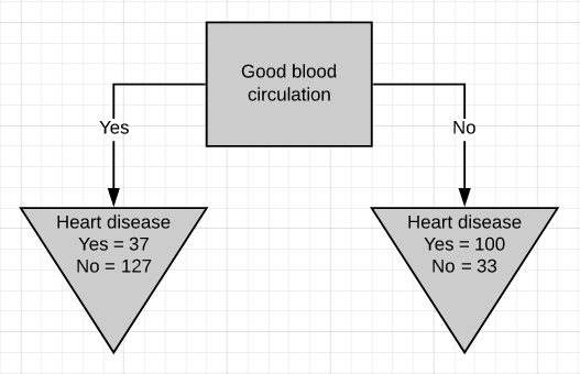
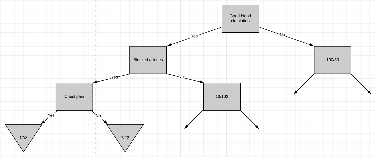
Gini impurity for ‘good blood circulation’ = 0.360Gini impurity for ‘blocked arteries’ = 0.381

‘Good blood circulation’ has the lowest impurity score among the tree which symbolizes that it best separates the patients having and not having heart disease, so we will use it at the root node.

“良好的血液循环”在树中具有最低的杂质评分，这表示它可以最好地区分患有和不患有心脏病的患者，因此我们将在根结点使用它。

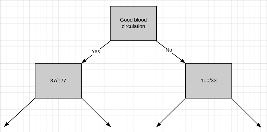
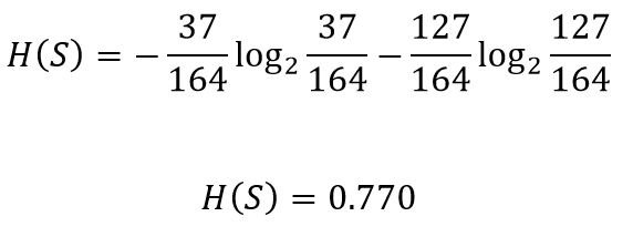
Now we need to figure out how well ‘chest pain’ and ‘blocked arteries’ separate the 164 patients in the left node(37 with heart disease and 127 without heart disease).

现在，我们需要弄清楚“胸痛”和“动脉阻塞”对左结的164例患者(37例有心脏病和127例无心脏病)的分隔情况。

Just like we did before we will separate these patients with ‘chest pain’ and calculate the Gini impurity value.

就像我们之前所做的那样，我们将这些患有“胸痛”的患者分开，并计算出基尼杂质值。

The Gini impurity was found to be 0.3. Then we do the same thing for ‘blocked arteries’.

发现基尼杂质为0.3。 然后，我们对“阻塞的动脉”执行相同的操作。

The Gini impurity was found to be 0.29. Since ‘blocked arteries’ has the lowest Gini impurity, we will use it at the left node in Fig.10 for further separating the patients.

发现基尼杂质为0.29。 由于“阻塞的动脉”具有最低的基尼杂质，因此我们将在图10的左侧节点使用它来进一步分离患者。

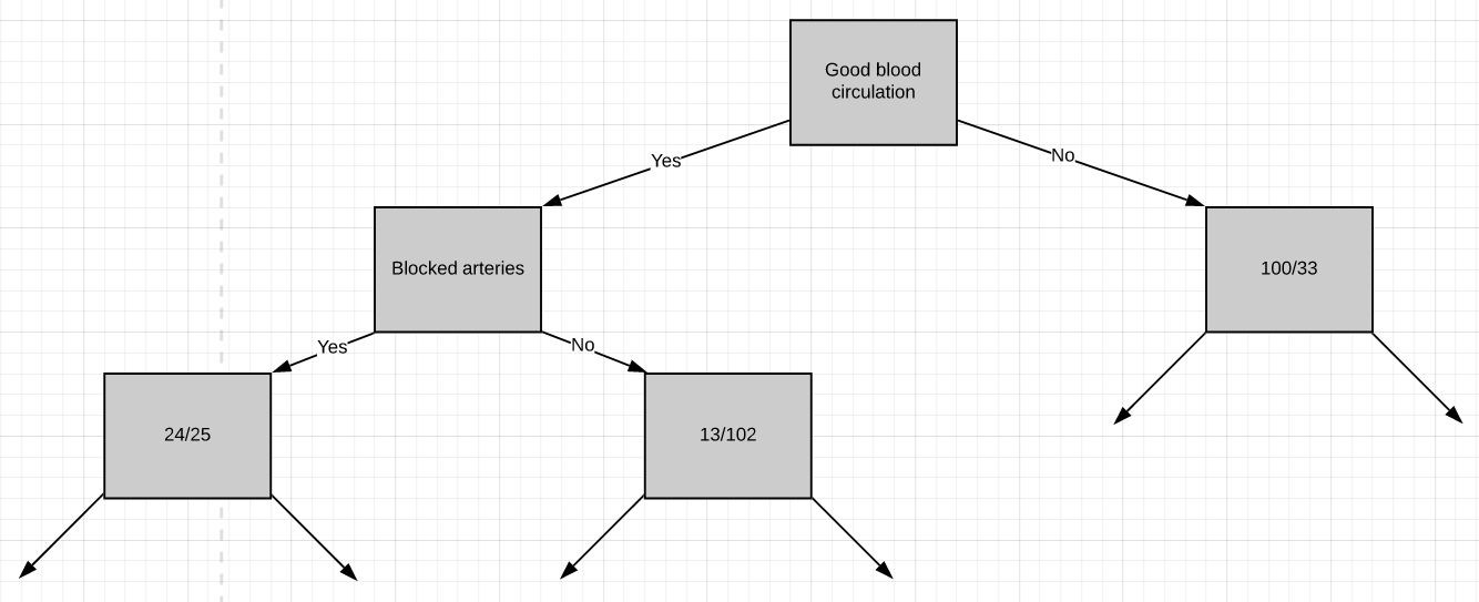
All we have left is ‘chest pain’, so we will see how well it separates the 49 patients in the left node(24 with heart disease and 25 without heart disease).

我们只剩下“胸痛”，因此我们将看到它如何很好地分隔了左结中的49位患者(24位有心脏病和25位无心脏病)。

We can see that chest pain does a good job separating the patients.

我们可以看到，胸痛在分隔患者方面做得很好。

So these are the final leaf nodes of the left side of this branch of the tree. Now let’s see what happens when we try to separate the node having 13/102 patients using ‘chest pain’. Note that almost 90% of the people in this node are not having heart disease.

因此，这些是树的此分支左侧的最终叶节点。 现在，让我们看看当尝试使用“胸痛”分离具有13/102个患者的节点时会发生什么。 请注意，此节点中几乎90％的人没有心脏病。

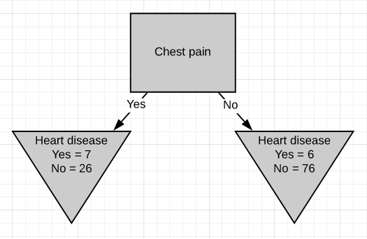
The Gini impurity of this separation is 0.29. But the Gini impurity for the parent-node before using chest-pain to separate the patients is

该分离的基尼杂质为0.29。 但是在使用胸痛将患者分开之前，父节点的基尼杂质是

Gini impurity = 1 - (probability of yes)² - (probability of no)²              = 1 - (13/13+102)² - (102/13+102)²Gini impurity = 0.2

The impurity is lower if we don’t separate patients using ‘chest pain’. So we will make it a leaf-node.

如果我们不使用“胸痛”将患者分开，那么杂质就更少。 因此，我们将其设为叶节点。

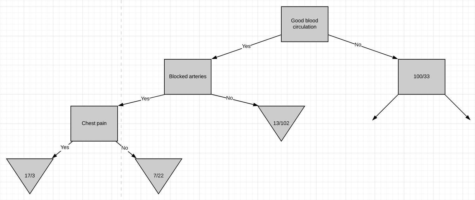
At this point, we have worked out the entire left side of the tree. The same steps are to be followed to work out the right side of the tree.

至此，我们已经算出了树的整个左侧。 遵循相同的步骤来计算树的右侧。

1. Calculate the Gini impurity scores.计算基尼杂质分数。
2. If the node itself has the lowest score, then there is no point in separating the patients anymore and it becomes a leaf node.如果节点本身的得分最低，则不再需要分离患者，而是成为叶节点。
3. If separating the data results in improvement then pick the separation with the lowest impurity value.如果分离数据可以改善质量，则选择杂质值最低的分离方法。

ID3 (ID3)

The process of building a decision tree using the ID3 algorithm is almost similar to using the CART algorithm except for the method used for measuring purity/impurity. The metric used in the ID3 algorithm to measure purity is called Entropy.

除了用于测量纯度/杂质的方法外，使用ID3算法构建决策树的过程几乎与使用CART算法相似。 ID3算法中用于测量纯度的度量标准称为熵 。

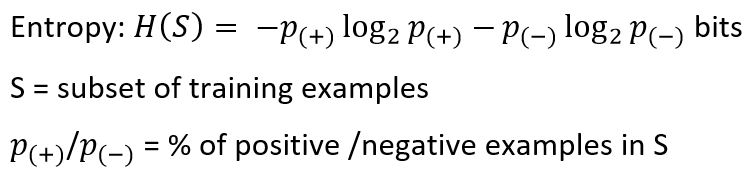
Entropy is a way to measure the uncertainty of a class in a subset of examples. Assume item belongs to subset S having two classes positive and negative. Entropy is defined as the no. of bits needed to say whether x is positive or negative.

熵是一种在子集中的示例中衡量类的不确定性的方法。 假设项属于具有正负两个类别的子集S。 熵定义为否。 需要说出x是正还是负的位。

Entropy always gives a number between 0 and 1. So if a subset formed after separation using an attribute is pure, then we will be needing zero bits to tell if is positive or negative. If the subset formed is having equal no. of positive and negative items then the no. of bits needed would be 1.

熵总是给出一个介于0和1之间的数字。因此，如果使用属性进行分离后形成的子集是纯净的，那么我们将需要零位来判断它是正还是负。 如果形成的子集具有相等的否。 积极和消极的项目，然后没有。 需要的位数为1。

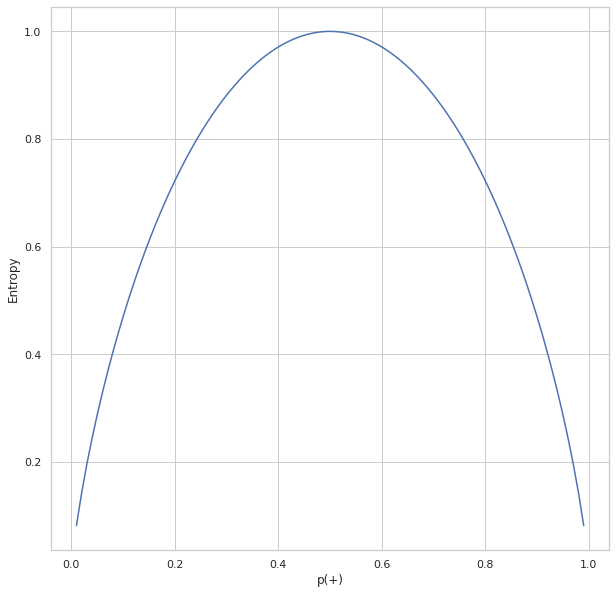
The above plot shows the relation between entropy and i.e., the probability of positive class. As we can see, the entropy reaches 1 which is the maximum value when which is there are equal chances for an item to be either positive or negative. The entropy is at its minimum when p(+) tends to zero(symbolizing x is negative) or 1(symbolizing x is positive).

上图显示了熵与正类别概率之间的关系。 正如我们所看到的，熵达到1时，这是最大值，当一个项目有相等的机会成为正数或负数时。 当p(+)趋于零(象征x为负)或1(象征x为正)时，熵处于最小值。

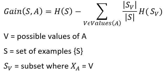
Entropy tells us how pure or impure each subset is after the split. What we need to do is aggregate these scores to check whether the split is feasible or not. This is done by Information gain.

熵告诉我们分割后每个子集的纯或不纯。 我们需要做的是汇总这些分数，以检查拆分是否可行。 这是通过信息获取来完成的。

Consider this part of the problem we discussed above for the CART algorithm. We need to decide which attribute to use from chest pain and blocked arteries for separating the left node containing 164 patients(37 having heart disease and 127 not having heart disease). We can calculate the entropy before splitting as

考虑上面我们针对CART算法讨论的问题的这一部分。 我们需要决定从chest pain和blocked arteries使用哪个属性来分离左结，该左结包含164位患者(37位患有心脏病和127位没有心脏病)。 我们可以在分解为

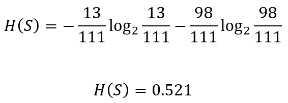
Let’s see how well chest pain separates the patients

让我们看看chest pain如何使患者分开

The entropy for the left node can be calculated

可以计算出左节点的熵

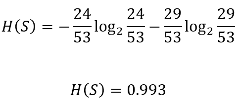
Similarly the entropy for the right node

类似地，右节点的熵

The total gain in entropy after splitting using chest pain

使用chest pain分裂后的总熵增加

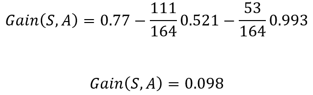
This implies that if in the current situation if we were to pick chest pain for splitting the patients, we would gain 0.098 bits in certainty on the patient having or not having heart disease. Doing the same for blocked arteries , the gain obtained was 0.117. Since splitting with blocked arteries gives us more certainty, it would be picked. We can repeat the same procedure for all the nodes to build a DT based on the ID3 algorithm.

这意味着，如果在当前情况下，如果我们为了让患者分担而chest pain ，那么在患有或没有心脏病的患者中，我们将获得0.098位的确定性。 对blocked arteries进行相同的操作，获得的增益为0.117。 由于blocked arteries分裂 给我们更多的确定性，它将被选中。 我们可以对所有节点重复相同的过程，以基于ID3算法构建DT。

Note: The decision of whether to split a node into 2 or to declare it as a leaf node can be made by imposing a minimum threshold on the gain value required. If the acquired gain is above the threshold value, we can split the node, otherwise, leave it as a leaf node.

注意：通过将最小阈值强加在所需的增益值上，可以决定是将节点拆分为2还是将其声明为叶节点。 如果获取的增益高于阈值，则可以拆分节点，否则将其保留为叶节点。

摘要 (Summary)

The following are the take-aways from this article

以下是本文的摘录

1. The general concept behind decision trees.决策树背后的一般概念。
2. The basic types of decision trees.决策树的基本类型。
3. Different algorithms to build a Decision tree.不同的算法来构建决策树。
4. Building a Decision tree using CART algorithm.使用CART算法构建决策树。
5. Building a Decision tree using ID3 algorithm.使用ID3算法构建决策树。