上文深度神经网络中各种优化算法原理及比较中介绍了深度学习中常见的梯度下降优化算法；其中，有一个重要的超参数——学习率\(\alpha\)需要在训练之前指定，学习率设定的重要性不言而喻：过小的学习率会降低网络优化的速度，增加训练时间；而过大的学习率则可能导致最后的结果不会收敛，或者在一个较大的范围内摆动；因此，在训练的过程中，根据训练的迭代次数调整学习率的大小，是非常有必要的；

  因此，本文主要介绍TensorFlow中如何使用学习率、TensorFlow中的几种学习率设置方式；文章中参考引用文献将不再具体文中说明，在文章末尾处会给出所有的引用文献链接；

  本主要主要介绍的学习率设置方式有：

• 指数衰减: tf.train.exponential_decay()
• 分段常数衰减: tf.train.piecewise_constant()
• 自然指数衰减: tf.train.natural_exp_decay()
• 多项式衰减tf.train.polynomial_decay()
• 倒数衰减tf.train.inverse_time_decay()
• 余弦衰减tf.train.cosine_decay()

1. 指数衰减

tf.train.exponential_decay(learning_rate,global_step, decay_steps, decay_rate,staircase=False, name=None):

参数	用法
learning_rate	初始学习率；
global_step	迭代次数；
decay_steps	衰减周期，当staircase=True时，学习率在\(decay\_steps\)内保持不变，即得到离散型学习率；
decay_rate	衰减率系数；
staircase	是否定义为离散型学习率，默认False；
name	名称，默认ExponentialDecay；

计算方式：

decayed_learning_rate = learning_rate * decay_rate ^ (global_step / decay_steps)
# 如果staircase=True，则学习率会在得到离散值，每decay_steps迭代次数，更新一次；

示例：

# coding:utf-8
import matplotlib.pyplot as plt
import tensorflow as tfglobal_step = tf.Variable(0, name='global_step', trainable=False) # 迭代次数y = []
z = []
EPOCH = 200with tf.Session() as sess:sess.run(tf.global_variables_initializer())for global_step in range(EPOCH):# 阶梯型衰减learing_rate1 = tf.train.exponential_decay(learning_rate=0.5, global_step=global_step, decay_steps=10, decay_rate=0.9, staircase=True)# 标准指数型衰减learing_rate2 = tf.train.exponential_decay(learning_rate=0.5, global_step=global_step, decay_steps=10, decay_rate=0.9, staircase=False)lr1 = sess.run([learing_rate1])lr2 = sess.run([learing_rate2])y.append(lr1)z.append(lr2)x = range(EPOCH)
fig = plt.figure()
ax = fig.add_subplot(111)
ax.set_ylim([0, 0.55])plt.plot(x, y, 'r-', linewidth=2)
plt.plot(x, z, 'g-', linewidth=2)
plt.title('exponential_decay')
ax.set_xlabel('step')
ax.set_ylabel('learing rate')
plt.legend(labels = ['staircase', 'continus'], loc = 'upper right')
plt.show()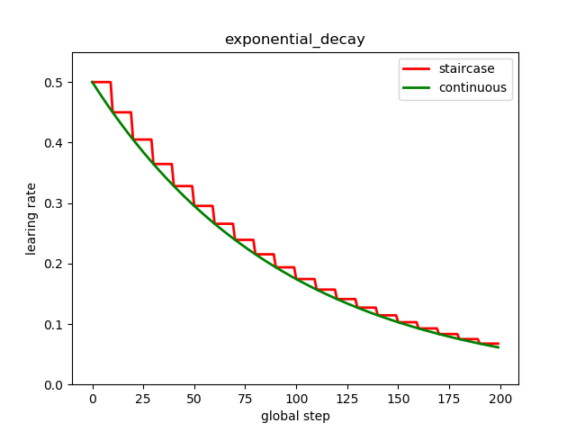

2. 分段常数衰减

tf.train.piecewise_constant(x, boundaries, values, name=None):

参数	用法
x	相当于global_step，迭代次数；
boundaries	列表，表示分割的边界；
values	列表，分段学习率的取值；
name	名称，默认PiecewiseConstant；

计算方式：

# parameter
global_step = tf.Variable(0, trainable=False)
boundaries = [100, 200]
values = [1.0, 0.5, 0.1]
# learning_rate
learning_rate = tf.train.piecewise_constant(global_step, boundaries, values)
# 解释
# 当global_step=[1, 100]时，learning_rate=1.0;
# 当global_step=[101, 200]时，learning_rate=0.5;
# 当global_step=[201, ~]时，learning_rate=0.1;

示例：

# coding:utf-8import matplotlib.pyplot as plt
import tensorflow as tfglobal_step = tf.Variable(0, name='global_step', trainable=False)
boundaries = [10, 20, 30]
learing_rates = [0.1, 0.07, 0.025, 0.0125]y = []
N = 40with tf.Session() as sess:sess.run(tf.global_variables_initializer())for global_step in range(N):learing_rate = tf.train.piecewise_constant(global_step, boundaries=boundaries, values=learing_rates)lr = sess.run([learing_rate])y.append(lr)x = range(N)
plt.plot(x, y, 'r-', linewidth=2)
plt.title('piecewise_constant')
plt.show()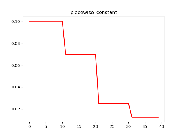

3. 自然指数衰减

类似与指数衰减，同样与当前迭代次数相关，只不过以e为底；

tf.train.natural_exp_decay(learning_rate,global_step,decay_steps,decay_rate,staircase=False,name=None
)

参数	用法
learning_rate	初始学习率；
global_step	迭代次数；
decay_steps	衰减周期，当staircase=True时，学习率在\(decay\_steps\)内保持不变，即得到离散型学习率；
decay_rate	衰减率系数；
staircase	是否定义为离散型学习率，默认False；
name	名称，默认ExponentialTimeDecay；

计算方式：

decayed_learning_rate = learning_rate * exp(-decay_rate * global_step)
# 如果staircase=True，则学习率会在得到离散值，每decay_steps迭代次数，更新一次；

示例：

# coding:utf-8import matplotlib.pyplot as plt
import tensorflow as tfglobal_step = tf.Variable(0, name='global_step', trainable=False)y = []
z = []
w = []
m = []
EPOCH = 200with tf.Session() as sess:sess.run(tf.global_variables_initializer())for global_step in range(EPOCH):# 阶梯型衰减learing_rate1 = tf.train.natural_exp_decay(learning_rate=0.5, global_step=global_step, decay_steps=10, decay_rate=0.9, staircase=True)# 标准指数型衰减learing_rate2 = tf.train.natural_exp_decay(learning_rate=0.5, global_step=global_step, decay_steps=10, decay_rate=0.9, staircase=False)# 阶梯型指数衰减learing_rate3 = tf.train.exponential_decay(learning_rate=0.5, global_step=global_step, decay_steps=10, decay_rate=0.9, staircase=True)# 标准指数衰减learing_rate4 = tf.train.exponential_decay(learning_rate=0.5, global_step=global_step, decay_steps=10, decay_rate=0.9, staircase=False)lr1 = sess.run([learing_rate1])lr2 = sess.run([learing_rate2])lr3 = sess.run([learing_rate3])lr4 = sess.run([learing_rate4])y.append(lr1)z.append(lr2)w.append(lr3)m.append(lr4)x = range(EPOCH)
fig = plt.figure()
ax = fig.add_subplot(111)
ax.set_ylim([0, 0.55])plt.plot(x, y, 'r-', linewidth=2)
plt.plot(x, z, 'g-', linewidth=2)
plt.plot(x, w, 'r--', linewidth=2)
plt.plot(x, m, 'g--', linewidth=2)plt.title('natural_exp_decay')
ax.set_xlabel('step')
ax.set_ylabel('learing rate')
plt.legend(labels = ['natural_staircase', 'natural_continus', 'staircase', 'continus'], loc = 'upper right')
plt.show()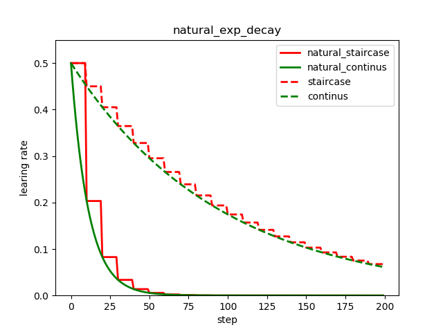

可以看到自然指数衰减对学习率的衰减程度远大于一般的指数衰减；

4. 多项式衰减

tf.train.polynomial_decay(learning_rate, global_step, decay_steps,end_learning_rate=0.0001, power=1.0,cycle=False, name=None):

参数	用法
learning_rate	初始学习率；
global_step	迭代次数；
decay_steps	衰减周期；
end_learning_rate	最小学习率，默认0.0001；
power	多项式的幂，默认1；
cycle	bool，表示达到最低学习率时，是否升高再降低，默认False；
name	名称，默认PolynomialDecay；

计算方式：

# 如果cycle=False
global_step = min(global_step, decay_steps)
decayed_learning_rate = (learning_rate - end_learning_rate) *(1 - global_step / decay_steps) ^ (power) +end_learning_rate
# 如果cycle=True
decay_steps = decay_steps * ceil(global_step / decay_steps)
decayed_learning_rate = (learning_rate - end_learning_rate) *(1 - global_step / decay_steps) ^ (power) +end_learning_rate

示例：

# coding:utf-8
import matplotlib.pyplot as plt
import tensorflow as tfy = []
z = []
EPOCH = 200global_step = tf.Variable(0, name='global_step', trainable=False)with tf.Session() as sess:sess.run(tf.global_variables_initializer())for global_step in range(EPOCH):# cycle=Falselearing_rate1 = tf.train.polynomial_decay(learning_rate=0.1, global_step=global_step, decay_steps=50,end_learning_rate=0.01, power=0.5, cycle=False)# cycle=Truelearing_rate2 = tf.train.polynomial_decay(learning_rate=0.1, global_step=global_step, decay_steps=50,end_learning_rate=0.01, power=0.5, cycle=True)lr1 = sess.run([learing_rate1])lr2 = sess.run([learing_rate2])y.append(lr1)z.append(lr2)x = range(EPOCH)
fig = plt.figure()
ax = fig.add_subplot(111)
plt.plot(x, z, 'g-', linewidth=2)
plt.plot(x, y, 'r--', linewidth=2)
plt.title('polynomial_decay')
ax.set_xlabel('step')
ax.set_ylabel('learing rate')
plt.legend(labels=['cycle=True', 'cycle=False'], loc='uppper right')
plt.show()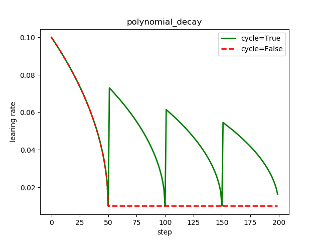

可以看到学习率在decay_steps=50迭代次数后到达最小值；同时，当cycle=False时，学习率达到预设的最小值后，就保持最小值不再变化；当cycle=True时，学习率将会瞬间增大，再降低；

多项式衰减中设置学习率可以往复升降的目的：时为了防止在神经网络训练后期由于学习率过小，导致网络参数陷入局部最优，将学习率升高，有可能使其跳出局部最优；

5. 倒数衰减

inverse_time_decay(learning_rate,global_step,decay_steps,decay_rate,staircase=False,name=None):

参数	用法
learning_rate	初始学习率；
global_step	迭代次数；
decay_steps	衰减周期；
decay_rate	学习率衰减参数；
staircase	是否得到离散型学习率，默认False；
name	名称；默认InverseTimeDecay；

计算方式：

# 如果staircase=False，即得到连续型衰减学习率；
decayed_learning_rate = learning_rate / (1 + decay_rate * global_step / decay_step)# 如果staircase=True，即得到离散型衰减学习率；
decayed_learning_rate = learning_rate / (1 + decay_rate * floor(global_step / decay_step))

示例：

# coding:utf-8import matplotlib.pyplot as plt
import tensorflow as tfy = []
z = []
EPOCH = 200
global_step = tf.Variable(0, name='global_step', trainable=False)with tf.Session() as sess:sess.run(tf.global_variables_initializer())for global_step in range(EPOCH):# 阶梯型衰减learing_rate1 = tf.train.inverse_time_decay(learning_rate=0.1, global_step=global_step, decay_steps=20,decay_rate=0.2, staircase=True)# 连续型衰减learing_rate2 = tf.train.inverse_time_decay(learning_rate=0.1, global_step=global_step, decay_steps=20,decay_rate=0.2, staircase=False)lr1 = sess.run([learing_rate1])lr2 = sess.run([learing_rate2])y.append(lr1)z.append(lr2)x = range(EPOCH)
fig = plt.figure()
ax = fig.add_subplot(111)
plt.plot(x, z, 'r-', linewidth=2)
plt.plot(x, y, 'g-', linewidth=2)
plt.title('inverse_time_decay')
ax.set_xlabel('step')
ax.set_ylabel('learing rate')
plt.legend(labels=['continus', 'staircase'])
plt.show()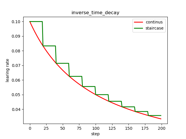

同样可以看到，随着迭代次数的增加，学习率在逐渐减小，同时减小的幅度也在降低；

6. 余弦衰减

之前使用TensorFlow的版本是1.4，没有学习率的余弦衰减；之后升级到了1.9版本，发现多了四个有关学习率余弦衰减的方法；下面将进行介绍：

6.1 标准余弦衰减

来源于：[Loshchilov & Hutter, ICLR2016], SGDR: Stochastic Gradient Descent with Warm Restarts. https://arxiv.org/abs/1608.03983

tf.train.cosine_decay(learning_rate, global_step, decay_steps, alpha=0.0, name=None):

参数	用法
learning_rate	初始学习率；
global_step	迭代次数；
decay_steps	衰减周期；
alpha	最小学习率，默认为0；
name	名称，默认CosineDecay；

计算方式：

global_step = min(global_step, decay_steps)
cosine_decay = 0.5 * (1 + cos(pi * global_step / decay_steps))
decayed = (1 - alpha) * cosine_decay + alpha
decayed_learning_rate = learning_rate * decayed

示例：

# coding:utf-8
import matplotlib.pyplot as plt
import tensorflow as tfy = []
z = []
EPOCH = 200
global_step = tf.Variable(0, name='global_step', trainable=False)with tf.Session() as sess:sess.run(tf.global_variables_initializer())for global_step in range(EPOCH):# 余弦衰减learing_rate1 = tf.train.cosine_decay(learning_rate=0.1, global_step=global_step, decay_steps=50)learing_rate2 = tf.train.cosine_decay(learning_rate=0.1, global_step=global_step, decay_steps=100)lr1 = sess.run([learing_rate1])lr2 = sess.run([learing_rate2])y.append(lr1)z.append(lr2)x = range(EPOCH)
fig = plt.figure()
ax = fig.add_subplot(111)
plt.plot(x, y, 'r-', linewidth=2)
plt.plot(x, z, 'b-', linewidth=2)
plt.title('cosine_decay')
ax.set_xlabel('step')
ax.set_ylabel('learing rate')
plt.legend(labels=['decay_steps=50', 'decay_steps=100'],z loc='upper right')
plt.show()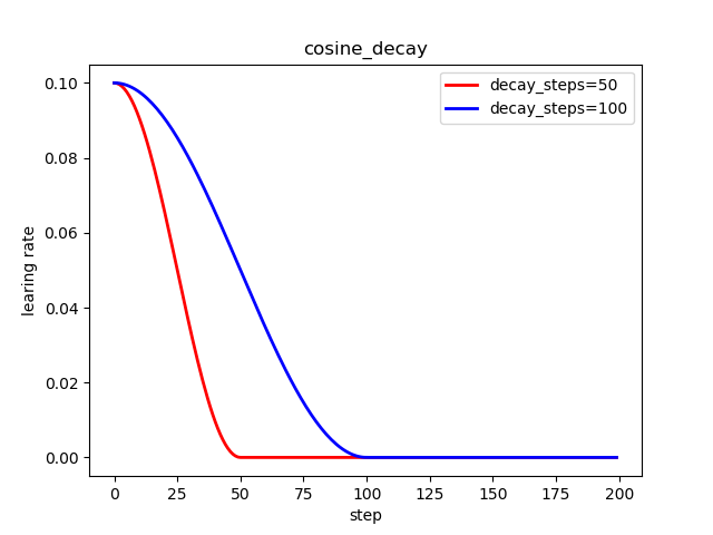

6.2 重启余弦衰减

来源于：[Loshchilov & Hutter, ICLR2016], SGDR: Stochastic Gradient Descent with Warm Restarts. https://arxiv.org/abs/1608.03983

tf.train.cosine_decay_restarts(learning_rate,global_step,first_decay_steps,t_mul=2.0,m_mul=1.0,alpha=0.0,name=None):

参数	用法
learning_rate	初始学习率；
global_step	迭代次数；
first_decay_steps	衰减周期；
t_mul	Used to derive the number of iterations in the i-th period
m_mul	Used to derive the initial learning rate of the i-th period:
alpha	最小学习率，默认为0；
name	名称，默认SGDRDecay；

示例：

# coding:utf-8
import matplotlib.pyplot as plt
import tensorflow as tfy = []
z = []
EPOCH = 100
global_step = tf.Variable(0, name='global_step', trainable=False)with tf.Session() as sess:sess.run(tf.global_variables_initializer())for global_step in range(EPOCH):# 重启余弦衰减learing_rate1 = tf.train.cosine_decay_restarts(learning_rate=0.1, global_step=global_step,first_decay_steps=40)learing_rate2 = tf.train.cosine_decay_restarts(learning_rate=0.1, global_step=global_step,first_decay_steps=60)lr1 = sess.run([learing_rate1])lr2 = sess.run([learing_rate2])y.append(lr1)z.append(lr2)x = range(EPOCH)
fig = plt.figure()
ax = fig.add_subplot(111)
plt.plot(x, y, 'r-', linewidth=2)
plt.plot(x, z, 'b-', linewidth=2)
plt.title('cosine_decay')
ax.set_xlabel('step')
ax.set_ylabel('learing rate')
plt.legend(labels=['decay_steps=40', 'decay_steps=60'], loc='upper right')
plt.show()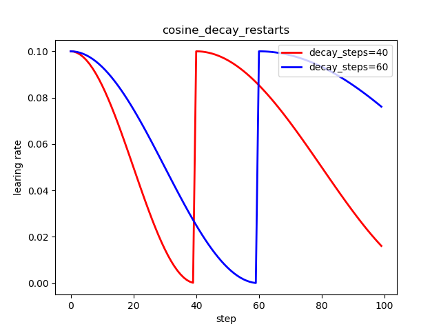

6.3 线性余弦噪声

来源于：[Bello et al., ICML2017] Neural Optimizer Search with RL. https://arxiv.org/abs/1709.07417

tf.train.linear_cosine_decay(learning_rate,global_step,decay_steps,num_periods=0.5,alpha=0.0,beta=0.001,name=None):

参数	用法
learning_rate	初始学习率；
global_step	迭代次数；
decay_steps	衰减周期；
num_periods	Number of periods in the cosine part of the decay.
alpha	最小学习率；
beta	同上；
name	名称，

计算方式：

global_step = min(global_step, decay_steps)
linear_decay = (decay_steps - global_step) / decay_steps)
cosine_decay = 0.5 * (1 + cos(pi * 2 * num_periods * global_step / decay_steps))
decayed = (alpha + linear_decay) * cosine_decay + beta
decayed_learning_rate = learning_rate * decayed

示例：

# coding:utf-8
import matplotlib.pyplot as plt
import tensorflow as tfy = []
z = []
EPOCH = 100
global_step = tf.Variable(0, name='global_step', trainable=False)with tf.Session() as sess:sess.run(tf.global_variables_initializer())for global_step in range(EPOCH):# 线性余弦衰减learing_rate1 = tf.train.linear_cosine_decay(learning_rate=0.1, global_step=global_step, decay_steps=40,num_periods=0.2, alpha=0.5, beta=0.2)learing_rate2 = tf.train.linear_cosine_decay(learning_rate=0.1, global_step=global_step, decay_steps=60,num_periods=0.2, alpha=0.5, beta=0.2)lr1 = sess.run([learing_rate1])lr2 = sess.run([learing_rate2])y.append(lr1)z.append(lr2)x = range(EPOCH)
fig = plt.figure()
ax = fig.add_subplot(111)
plt.plot(x, y, 'r-', linewidth=2)
plt.plot(x, z, 'b-', linewidth=2)
plt.title('linear_cosine_decay')
ax.set_xlabel('step')
ax.set_ylabel('learing rate')
plt.legend(labels=['decay_steps=40', 'decay_steps=60'], loc='upper right')
plt.show()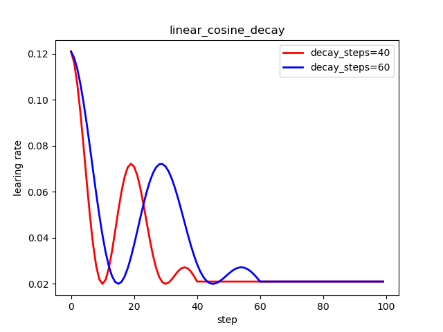

6.4 噪声余弦衰减

来源于：[Bello et al., ICML2017] Neural Optimizer Search with RL. https://arxiv.org/abs/1709.07417

tf.train.noisy_linear_cosine_decay(learning_rate,global_step,decay_steps,initial_variance=1.0,variance_decay=0.55,num_periods=0.5,alpha=0.0,beta=0.001,name=None):

参数	用法
learning_rate	初始学习率；
global_step	迭代次数；
decay_steps	衰减周期；
initial_variance	initial variance for the noise.
variance_decay	decay for the noise's variance.
num_periods	Number of periods in the cosine part of the decay.
alpha	最小学习率；
beta	查看计算公式；
name	名称，默认NoisyLinearCosineDecay；

计算方式：

global_step = min(global_step, decay_steps)
linear_decay = (decay_steps - global_step) / decay_steps)
cosine_decay = 0.5 * (1 + cos(pi * 2 * num_periods * global_step / decay_steps))
decayed = (alpha + linear_decay + eps_t) * cosine_decay + beta
decayed_learning_rate = learning_rate * decayed

示例：

# coding:utf-8
import matplotlib.pyplot as plt
import tensorflow as tfy = []
z = []
EPOCH = 100
global_step = tf.Variable(0, name='global_step', trainable=False)with tf.Session() as sess:sess.run(tf.global_variables_initializer())for global_step in range(EPOCH):# # 噪声线性余弦衰减learing_rate1 = tf.train.noisy_linear_cosine_decay(learning_rate=0.1, global_step=global_step, decay_steps=40,initial_variance=0.01, variance_decay=0.1, num_periods=2, alpha=0.5, beta=0.2)learing_rate2 = tf.train.noisy_linear_cosine_decay(learning_rate=0.1, global_step=global_step, decay_steps=60,initial_variance=0.01, variance_decay=0.1, num_periods=2, alpha=0.5, beta=0.2)lr1 = sess.run([learing_rate1])lr2 = sess.run([learing_rate2])y.append(lr1)z.append(lr2)x = range(EPOCH)
fig = plt.figure()
ax = fig.add_subplot(111)
plt.plot(x, y, 'r-', linewidth=2)
plt.plot(x, z, 'b-', linewidth=2)
plt.title('noisy_linear_cosine_decay')
ax.set_xlabel('step')
ax.set_ylabel('learing rate')
plt.legend(labels=['decay_steps=40', 'decay_steps=60'], loc='upper right')
plt.show()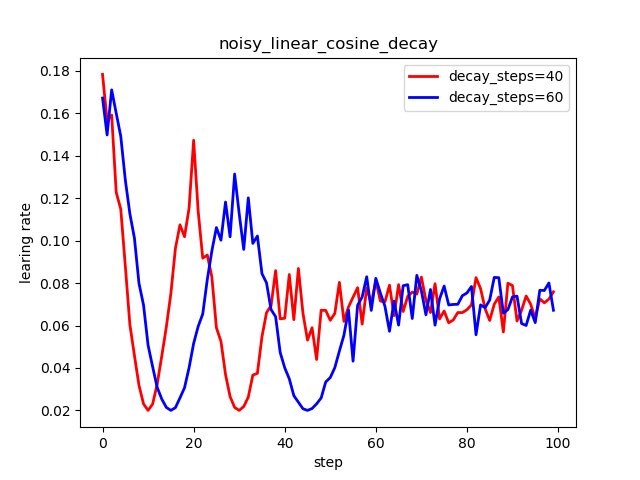

 写在最后，将TensorFlow中提供的所有学习率衰减的方式大致地使用了一遍，突然发现，掌握的也仅仅是TensorFlow中提供了哪些衰减方式、大致如何使用；然而，当涉及到某种具体的衰减方式、参数如何设置与背后的数学意义，以及不同的方法适用于什么情况....等等一些问题，仍不能掌握。如有可能，在之后使用的过程中，当发现有新的理解，再回来补充。

  如有错误，请不吝指正，谢谢。

  这里感谢未雨愁眸-tensorflow中学习率更新策略的博文，本文主要参考该篇文章；当然在其他地方也有看到类似文章，至于说首发何人何处，却未从考证；

博主个人网站：https://chenzhen.onliine

Reference

• 未雨愁眸-tensorflow中学习率更新策略