SQL Server中的基数估计过程
In this post, we are going to take a deeper look at the cardinality estimation process. We will use SQL Server 2014, the main concepts might also be applied to the earlier versions, however, the process details are different.
在本文中,我们将更深入地了解基数估计过程。 我们将使用SQL Server 2014,主要概念也可能会应用于早期版本,但是过程细节有所不同。
计算器 (Calculators)
The algorithms responsible for performing the cardinality estimation in SQL Server 2014 are implemented in the classes called Calculators.
SQL Server 2014中负责执行基数估计的算法在称为计算器的类中实现。
CSelCalc – Class Selectivity Calculator.
CSelCalc –类选择性计算器。
CDVC – Class Distinct Value Calculator.
CDVC –类区别值计算器。
To be more specific, these classes might not contain the one estimation algorithm, rather they join together a set of specific algorithms and drive them. For example calculator CSelCalcExpressionComparedToExpression may estimate join cardinality using join columns histograms in a different ways, depending on the model variation, and the specific estimation algorithms are implemented in the different classes, used by this calculator.
更具体地说,这些类可能不包含一个估计算法,而是将一组特定算法结合在一起并对其进行驱动。 例如,计算器CSelCalcExpressionComparedToExpression可以根据模型变化,以不同方式使用连接列直方图来估计连接基数,并且特定的估计算法是在此计算器使用的不同类中实现的。
I mentioned a model variation – this is another new concept in the new cardinality estimation framework. One of the goals of implementing the new cardinality estimation mechanism was to achieve more flexibility and control over the estimation process. Different workload types demand different approaches to the estimation and there are some special cases when two approaches may contradict each other. Model variations are based on a mechanism of pluggable heuristics and may be used in special cases.
我提到了一个模型变体–这是新的基数估计框架中的另一个新概念。 实施新的基数估计机制的目标之一是实现更大的灵活性并控制估计过程。 不同的工作量类型需要不同的估算方法,并且在某些特殊情况下,两种方法可能会相互矛盾。 模型变化基于可插入启发式机制,并且可能在特殊情况下使用。
SQL Server 2014 has additional diagnostic mechanisms which allow us to take a closer look at how the estimation process works. These are trace flag 2363 and extended event query_optimizer_cardinality_estimation. They might be used together to get the maximum of the estimation process details.
SQL Server 2014具有其他诊断机制,使我们可以更仔细地了解估计过程的工作方式。 这些是跟踪标志2363和扩展事件query_optimizer_cardinality_estimation 。 可以将它们一起使用以获取最大的估计过程详细信息。
估算过程 (The Estimation Process)
Let’s consider a simple example of a query, in database “opt” , that selects from the table and filter rows.
让我们考虑一个简单的查询示例,在数据库“ opt”中,该查询从表中选择并过滤行。
use opt;
go
set showplan_xml on
go
select * from t1 where b = 100 option(querytraceon 9130)
go
set showplan_xml off
go
Note: Normally, the optimizer would join together a filter and a scan operator on the phase when the Physical Operators Tree is converted to the Plan Operators Tree (this process is known as Post Optimization Rewrite), to avoid a separate Filter plan operator and reduce the cost of passing rows between Filter and Scan operator. To prevent this, for demonstration purposes, I use trace flag 9130, that disables this particular rewrite.
注意:通常,当将物理运算符树转换为计划运算符树时,该优化程序会在阶段将过滤器和扫描运算符结合在一起(此过程称为后期优化重写),以避免单独的过滤器计划运算符并减少在筛选器和扫描运算符之间传递行的成本。 为了防止这种情况,出于演示目的,我使用了跟踪标志9130,该标志禁用了此特定的重写。
This query has the following simple plan:
该查询具有以下简单计划:
Let’s use the undocumented TF 2363, mentioned above, to view diagnostic output. We also use TF 8606, described in the previous post, to view logical operators tree with TF 8612 to add cardinality info. TF 3604 is also necessary to direct output to console.
让我们使用上面提到的未记录的TF 2363来查看诊断输出。 我们还使用上一篇文章中描述的TF 8606来查看带有TF 8612的逻辑运算符树,以添加基数信息。 TF 3604对于将输出定向到控制台也是必需的。
set showplan_xml on
go
select * from t1 where b = 100 option(querytraceon 9130, querytraceon 8606, querytraceon 8612, querytraceon 2363, querytraceon 3604)
go
set showplan_xml off
go
If we switch to the message tab, we’ll see the following output:
如果切换到消息选项卡,我们将看到以下输出:
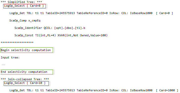
Between the two trees of the logical operators, there is some additional output that starts with the phrase “Begin selectivity computation” and ends with “End selectivity computation”. I copied this output to the image below and painted it, to give some explanations.
在逻辑运算符的两棵树之间,有一些附加输出,它们以短语“开始选择性计算”开头,以“结束选择性计算”结尾。 我将此输出复制到下面的图像并进行绘制,以给出一些解释。
The TF Output:
TF输出:
The Process:
流程:
The process starts with the input tree of logical operators. For that simple case there are only two of them:
该过程从逻辑运算符的输入树开始。 对于这种简单的情况,只有两个:
- LogOp_Get – gets the table LogOp_Get –获取表
- LogOp_Select – selects from the table, this is a relational select, that means “select from set”, i.e. filtering LogOp_Select –从表中选择,这是一个关系选择,表示“从集合中选择”,即过滤
- Scalar operators – determine the comparison condition, here we have an equality check for a column and a constant 标量运算符 –确定比较条件,这里我们对列和常量进行相等检查
The tree is depicted on the left of the second picture. The cardinality calculation goes bottom-up, starting from the lowest operator (or the up-right if we look at the graphical plan). In the diagnostic output, we see that a base table statistics collection was loaded for the lowest logical operator “get table”.
该树显示在第二张图片的左侧。 基数计算自下而上,从最低的运算符开始(如果我们查看图形计划,则从右至上)。 在诊断输出中,我们看到已为最低逻辑运算符“ get table”加载了基表统计信息集合。
Next, the filter selectivity should be computed. For that purpose, the plan for selectivity computation is selected, in our case, this would be the calculator – CSelCalcColumnInInterval. The one may ask, why “interval”, if there is an equality comparison. The answer is, that our column is not unique and so several rows are possible. If it had a unique constraint or index the calculator would be CSelCalcUniqueKeyFilter.
接下来,应计算过滤器的选择性。 为此,选择了选择性计算计划,在我们的示例中,这将是计算器– CSelCalcColumnInInterval。 一个人可能会问,为什么要进行“间隔”比较是否相等。 答案是,我们的列不是唯一的,因此可能有几行。 如果它具有唯一约束或索引,则计算器将为CSelCalcUniqueKeyFilter。
The calculator computes the selectivity using input statistics from the operator get (the output even tells us what histogram was loaded), and a set of algorithms, that represents this type of calculator and are based on the mathematical model, discussed in the previous post. The computed selectivity is 0.01.
计算器使用来自运算符get的输入统计信息(输出甚至告诉我们加载了直方图)和一组算法(代表这种类型的计算器并基于数学模型)计算选择性,该算法在上一篇文章中进行了讨论。 计算的选择性为0.01。
This selectivity is multiplied by the input cardinality of 1000 rows and we have an estimate: 1000*0.01 = 10 rows. Perfect!
此选择性乘以1000行的输入基数,我们得到一个估计:1000 * 0.01 = 10行。 完善!
The next step, takes this cardinality, modifies density and histogram according to it, and generates a new statistics collection – filter statistics collection. If we had a more complex plan, this statistics collection might be used as an input statistics for the next logical operator, which is higher than Filter, and so on. This process goes from bottom to top, until all the tree nodes will have an estimate.
下一步,采用该基数,根据其修改密度和直方图,并生成一个新的统计信息集合-过滤统计信息集合。 如果我们有一个更复杂的计划,则此统计信息集合可以用作下一个逻辑运算符的输入统计信息,该逻辑运算符高于Filter,依此类推。 此过程从下到上进行,直到所有树节点都有一个估计为止。
更复杂的例子 (More complex example)
The query below joins two tables, filters and groups data for the distinct purposes.
下面的查询将两个表连接起来,分别用于数据过滤和分组。
set showplan_xml on
go
select distinct t1.b, t2.b from t1 join t2 on t2.b = t1.b where t1.b < 300
option(recompile, merge join
, querytraceon 3604 -- <-- Output to Console
, querytraceon 8606 -- <-- Show LogOp Trees
, querytraceon 8619 -- <-- Show Applied Transformation Rules
, querytraceon 8612 -- <-- Add Extra Info to the Trees Output
, querytraceon 2363 -- <-- (2014, new:) TF Selectivity
);
go
set showplan_xml off
go
It has the following plan:
它有以下计划:
A few notes about this plan.
有关此计划的一些注意事项。
The DISTINCT clause is used in the query, that means only unique pairs of values t1.b and t2.b should be returned. To satisfy this, the server uses grouping by means of the operator Stream Aggregate. What is worth noting, that one of the grouping columns – column t2. b has a primary key defined, therefore, is unique, because of that, the server may not group by that column and leave only t1.b for the aggregation. That means that the aggregation could be safely done before the join, to reduce the number of joining rows.
查询中使用DISTINCT子句,这意味着仅返回值t1.b和t2.b的唯一对。 为满足此要求,服务器通过运算符Stream Aggregate使用分组。 值得注意的是,分组列之一-列t2。 b有一个定义的主键,因此是唯一的,因此,服务器可能不会按该列分组,而只留下t1.b进行聚合。 这意味着可以在连接之前安全地进行聚合,以减少连接行的数量。
We filter on the t1.b column and join on it also, so the filter could be applied to t2.b column also. The filter operator itself is not present in the plan as a separate plan operator, it is combined with a seek and scan.
我们在t1.b列上进行过滤并进行联接 ,因此该过滤器也可以应用于t2.b列。 筛选器运算符本身并不作为单独的计划运算符出现在计划中,而是与搜索和扫描结合使用。
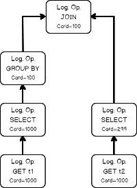
The logical operator tree for that query looks like this:
该查询的逻辑运算符树如下所示:
Let’s now watch, how goes the estimation process. I’ll not provide a TF diagnostic output here, because it is too verbose, rather, I’ll convert it into a graphical form, the series of pictures.
现在让我们来看一下估计过程。 我不会在这里提供TF诊断输出,因为它太冗长了,而是将其转换为图形形式的一系列图片。
The input tree of the logical operators, loading statistics collection of the base table.
逻辑运算符的输入树,加载基表的统计信息集合。

Estimating the filtering condition for column t1, as we saw in the previous simple example, and creating the new statistics collection.
如前面的简单示例所示,估计t1列的过滤条件,并创建新的统计信息集合。
- Doing the same thing with table t2, loading base statistics.对表t2做同样的事情,加载基本统计信息。
Estimating the filtering condition for t2.b (remember the filter was propagated, from t1.b because of the join equality comparison on the same column).
估计t2.b的过滤条件(由于同一列上的连接相等比较,请记住从t1.b传播了过滤器)。
Now we have all necessary input to estimate the join cardinality. Using filters statistics collection and the join calculator CSelCalcExpressionComparedToExpression to estimate the join cardinality. Note: in fact, the join may use base table statistics and combine it with a filter selectivity – this called Based Containment Assumption, but we will not delve into it here, because it’s worth a separate blog post.
现在,我们有了所有必要的输入来估计联接基数。 使用过滤器统计信息收集和联接计算器CSelCalcExpressionComparedToExpression估算联接基数。 注意:实际上,联接可能会使用基表统计信息并将其与过滤器选择性结合在一起-这称为“基于包含假设”,但是在这里我们将不对其进行深入研究,因为它值得单独撰写博客文章。
Finally, using the join statistics collection we are ready to calculate the cardinality of a grouping operation.
最后,使用联接统计信息收集,我们准备计算分组操作的基数。
Now we may set calculated cardinalities to the logical operator tree accordingly.
现在我们可以相应地将计算出的基数设置为逻辑运算符树。
At that moment we have the initial tree with set cardinalities. But as we remember from the previous post, the cardinality estimation occurs during the optimization process also, when the new logical group appears. This is the case. The optimizer decides that it will be beneficial to perform grouping before the join, to lower the number of joining rows. It applies the transformation rule, that generates the new alternative logical group and switches the Join and the Grouping (Group By Aggregate Before Join)..
到那时,我们有了具有设定基数的初始树。 但是,正如我们从上一篇文章中记得的那样,当出现新的逻辑组时,基数估计也会在优化过程中发生。 就是这种情况。 优化器认为在连接之前执行分组以减少连接行数将是有益的。 它应用转换规则,生成新的备用逻辑组并切换联接和分组(联接之前按聚集分组)。
The new group should also be estimated, because it’s cardinality is unknown.
还应该估计新组,因为基数未知。
The optimizer once again uses the input statistics of the child nodes.
优化器再次使用子节点的输入统计信息。
Using the same calculator CSelCalcExpressionComparedToExpression, the optimizer estimates the new logical group.
使用相同的计算器CSelCalcExpressionComparedToExpression,优化器估计新的逻辑组。
Now again, all the cardinalities are known.
再一次,所有基数都已知。
Later the logical Get and logical FIlter would be implemented as the Seek with a predicate and the Scan with a residual predicate, then the logical Join would be transformed to the physical Merge join and the group operator into the physical Stream Aggregate.
后来,将逻辑Get和逻辑过滤器实现为带有谓词的Seek和带有残差谓词的Scan,然后将逻辑Join转换为物理Merge连接,并将组运算符转换为物理Stream Aggregate。
That’s how it works!
这就是它的工作原理!
I’d like you to take out of this part one very important thing, that might be applied in practice. As you saw, the estimation goes from bottom to top, using child node statistics as an input to estimate a current node. If the estimation error appears at some step, it is propagated further, to the next operators. That’s why, when you try to struggle with inaccurate cardinality estimates, try to find the bottom most inaccurate estimate. Very likely it skewed all the next estimates. Don’t struggle with the top most inaccuracy, because this inaccuracy might be induced by the previous operators.
我希望您从这一部分中学到一件非常重要的事情,可以在实践中应用。 如您所见,使用子节点统计信息作为估计当前节点的输入,估计是从下到上进行的。 如果估计误差出现在某个步骤,它将进一步传播到下一个运算符。 这就是为什么当您尝试使用不准确的基数估计值时,请尝试找出最底端的最不正确的估计值。 它很可能会歪曲所有下一个估计。 不要与最不准确的地方作斗争,因为这种错误可能是由先前的操作员引起的。
For the truth, I should say, that sometimes there are curious cases, when the two incorrect estimates annihilate each other negative impact, and the plan is fine. If you eliminate one of them, the fragile balance is ruined and the plan becomes a problem. By the way, that is one of the reasons, why Microsoft was very conservative to introduce new changes to the cardinality estimation and left them “off” by default and demand a trace flag to use it.
实际上,我应该说,有时候会出现一些奇怪的情况,即两个错误的估计会相互抵消负面影响,并且计划是好的。 如果您消除其中之一,那么脆弱的平衡将被破坏,计划将成为问题。 顺便说一下,这就是原因之一,Microsoft为何非常保守地对基数估计进行新的更改,并默认将它们保留为“ off”,并要求使用跟踪标志。
In the next post we’ll see how the “old” cardinality estimation behavior may be used in SQL Server 2014.
在下一篇文章中,我们将看到如何在SQL Server 2014中使用“旧的”基数估计行为。
目录 (Table of Contents)
| Cardinality Estimation Role in SQL Server |
| Cardinality Estimation Place in the Optimization Process in SQL Server |
| Cardinality Estimation Concepts in SQL Server |
| Cardinality Estimation Process in SQL Server |
| Cardinality Estimation Framework Version Control in SQL Server |
| Filtered Stats and CE Model Variation in SQL Server |
| Join Containment Assumption and CE Model Variation in SQL Server |
| Overpopulated Primary Key and CE Model Variation in SQL Server |
| Ascending Key and CE Model Variation in SQL Server |
| MTVF and CE Model Variation in SQL Server |
| SQL Server中的基数估计角色 |
| 基数估计在SQL Server优化过程中的位置 |
| SQL Server中的基数估计概念 |
| SQL Server中的基数估计过程 |
| SQL Server中的基数估计框架版本控制 |
| SQL Server中的筛选后的统计信息和CE模型变化 |
| 在SQL Server中加入包含假设和CE模型变化 |
| SQL Server中人口过多的主键和CE模型的变化 |
| SQL Server中的升序密钥和CE模型变化 |
| SQL Server中的MTVF和CE模型变化 |
参考资料 (References)
- Cardinality Estimation (SQL Server) 基数估计(SQL Server)
- Testing cardinality estimation models in SQL server 在SQL Server中测试基数估计模型
- What’s New (Database Engine, SQL Server 2014) 新增功能(数据库引擎,SQL Server 2014)
翻译自: https://www.sqlshack.com/cardinality-estimation-process/
SQL Server中的基数估计过程相关推荐
- SQL Server中的基数估计角色
This post opens a series of blog posts dedicated to my observations of the new cardinality estimator ...
- sql判断基数_SQL Server中的基数估计框架版本控制
sql判断基数 This is a small post about how you may control the cardinality estimator version and determi ...
- SQL Server中的筛选后的统计信息和CE模型变化
In this blog post, we are going to view some interesting model variation, that I've found while expl ...
- 在SQL Server中加入包含假设和CE模型变化
In this post we are going to talk about one of the model assumptions, that was changed in the new ca ...
- SQL Server中的MTVF和CE模型变化
This is a note about multi-statement table valued functions (MTVF) and how their cardinality is esti ...
- 在AWS RDS SQL Server中恢复数据
This article explores the process to recover data in AWS RDS SQL Server and its recent enhancements. ...
- SQL Server 中的事务与事务隔离级别以及如何理解脏读, 未提交读,不可重复读和幻读产生的过程和原因...
原本打算写有关 SSIS Package 中的事务控制过程的,但是发现很多基本的概念还是需要有 SQL Server 事务和事务的隔离级别做基础铺垫.所以花了点时间,把 SQL Server 数据库中 ...
- SQL Server中并行执行计划的基础
In this article, we will learn the basics of Parallel Execution Plans, and we will also figure out h ...
- SQL Server中的万圣节问题和建议的解决方案
描述 (Description) As per Wikipedia, the Halloween problem was first discovered by Don Chamberlin, Pat ...
最新文章
- CompletableFuture 创建异步对象
- mysql解压缩版配置_MySQL 5.6 for Windows 解压缩版配置安装
- Bit.com BCH期权上线以来日交易量持续翻倍
- java 构造函数 和 构造代码块
- git分支创建分支删除分支合并
- linkedin android,如何在android中登录linkedin?
- 网站流量日志分析系统笔记(Hadoop大数据技术原理与应用)
- 打开UG10 C语言错误,修复UG软件在win10中出现运行乱码的错误方法
- 同济版《线性代数》再遭口诛笔伐,网友:它真的不太行
- 标准gpx文件的时间格式
- linux线程互踩,IOS 多线程漫漫谈(Process and Thread)
- 企业图纸共享办公系统哪个好
- 从小白开始教你怎样在Eclipse中使用Git(番外) - 各种图标的含义
- ai皮肤检测分数_你的皮肤好坏,之后可要AI机器人说了算,5秒钟检测出皮肤质量...
- B站最全Redis教程全集(2021最新版)(图灵学院诸葛)学习笔记一--五种数据结构与应用场景
- 陈艾盐:《春燕》百集访谈节目第三十九集
- BAT前端老鸟总结:未来几年web前端发展四大趋势前瞻
- shui0418笔记
- 聊聊国外LEAD最近一些情况
- 读论文|基于大平面物体垂直姿态的双向人机双手交接