Ceres Solver: 高效的非线性优化库（二）实战篇

接上篇: Ceres Solver: 高效的非线性优化库（一）

如何求导

Ceres Solver提供了一种自动求导的方案，上一篇我们已经看到。
但有些情况，不能使用自动求导方案。另外两种方案：解析求导和数值求导。

1. 解析求导

有些情况无法定义模板代价函数。比如残差函数是库函数，你无法知道。此时我们可以构建一个NumericDiffCostFunction，例如\[f(x)=10-x\].上面的例子变成

struct NumericDiffCostFunctor {bool operator()(const double* const x, double* residual) const {residual[0] = 10.0 - x[0];return true;}};
加入Problem中。
CostFunction* cost_function =new NumericDiffCostFunction<NumericDiffCostFunctor, ceres::CENTRAL, 1, 1>(new NumericDiffCostFunctor);
problem.AddResidualBlock(cost_function, NULL, &x);

同自动求导的区别

CostFunction* cost_function =new AutoDiffCostFunction<CostFunctor, 1, 1>(new CostFunctor);problem.AddResidualBlock(cost_function, NULL, &x);

一般而言，我们推荐自动求导，不适用数值求导。C++模板让自动求导非常高效，但解析求导速度很慢，且容易造成数值错误，收敛较慢。

2. 数值求导

有些情况，自动求导并不能使用。比如，有时候使用最终形势比自动求导的链式法则（chain rule）更方便。
这种情况下，需要提供残差和雅克比值。为此，我们需要定义一个CostFunction的子类（如果你知道残差在编译时的大小，可定义SizedCostFunction的子类）。下面依旧是\(f(x) = 10 - x\)的例子。

class QuadraticCostFunction : public ceres::SizedCostFunction<1, 1> {public:virtual ~QuadraticCostFunction() {}virtual bool Evaluate(double const* const* parameters,double* residuals,double** jacobians) const {const double x = parameters[0][0];residuals[0] = 10 - x;// Compute the Jacobian if asked for.if (jacobians != NULL && jacobians[0] != NULL) {jacobians[0][0] = -1;}return true;}};

SimpleCostFunction::Evaluate是输入参数，residuals是jacobian的输出。Jacobians是可选项，Evaluate用来检测它是否非空，否则帮它填充好。此示例下残差是线性的，雅克比是固定值。
这个方案是比较繁琐的。除非有必要，推荐使用AutoDiffCostFunction或NumericDiffCostFunction来创建。

3. 更多关于求导的内容

求导是目前Ceres Solver最复杂的内容，有时候用户需要根据情况旋转更方便的方案。本节只是大致介绍求导方案。熟悉Numeric和Auto之后，推荐了解DynamicAuto，CostFunctionToFunctor，NumericDiffFunctor和ConditionedCostFunction。

实战之Powell’s Function(一个稍微复杂点的例子)

考虑变量\[x = \left[x_1, x_2, x_3, x_4 \right]\]和
\[ \begin{split}\begin{align} f_1(x) &= x_1 + 10x_2 \\ f_2(x) &= \sqrt{5} (x_3 - x_4)\\ f_3(x) &= (x_2 - 2x_3)^2\\ f_4(x) &= \sqrt{10} (x_1 - x_4)^2\\ F(x) &= \left[f_1(x),\ f_2(x),\ f_3(x),\ f_4(x) \right] \end{align}\end{split} \]

$ F(x) \(是4个参数的函数，有4个残差，我们希望找到一个最小化\)\frac{1}{2}|F(x)|^2\(的变量\)x\(。第一步，定义一个衡量目标函数的算子。对于\)f_4(x_1, x_4)$:

struct F4 {template <typename T>bool operator()(const T* const x1, const T* const x4, T* residual) const {residual[0] = T(sqrt(10.0)) * (x1[0] - x4[0]) * (x1[0] - x4[0]);return true;}
};

类似的我们可以定义F1，F2，F3。利用这些算子，优化问题可使用下面的方法解决：

double x1 =  3.0; double x2 = -1.0; double x3 =  0.0; double x4 = 1.0;Problem problem;// Add residual terms to the problem using the using the autodiff
// wrapper to get the derivatives automatically.
problem.AddResidualBlock(new AutoDiffCostFunction<F1, 1, 1, 1>(new F1), NULL, &x1, &x2);
problem.AddResidualBlock(new AutoDiffCostFunction<F2, 1, 1, 1>(new F2), NULL, &x3, &x4);
problem.AddResidualBlock(new AutoDiffCostFunction<F3, 1, 1, 1>(new F3), NULL, &x2, &x3)
problem.AddResidualBlock(new AutoDiffCostFunction<F4, 1, 1, 1>(new F4), NULL, &x1, &x4);

对于每个ResidualBlock仅仅依赖2个变量。运行examples/powell.cc可以得到相应优化结果。

Initial x1 = 3, x2 = -1, x3 = 0, x4 = 1
iter      cost      cost_change  |gradient|   |step|    tr_ratio  tr_radius  ls_iter  iter_time  total_time0  1.075000e+02    0.00e+00    1.55e+02   0.00e+00   0.00e+00  1.00e+04       0    4.95e-04    2.30e-031  5.036190e+00    1.02e+02    2.00e+01   2.16e+00   9.53e-01  3.00e+04       1    4.39e-05    2.40e-032  3.148168e-01    4.72e+00    2.50e+00   6.23e-01   9.37e-01  9.00e+04       1    9.06e-06    2.43e-033  1.967760e-02    2.95e-01    3.13e-01   3.08e-01   9.37e-01  2.70e+05       1    8.11e-06    2.45e-034  1.229900e-03    1.84e-02    3.91e-02   1.54e-01   9.37e-01  8.10e+05       1    6.91e-06    2.48e-035  7.687123e-05    1.15e-03    4.89e-03   7.69e-02   9.37e-01  2.43e+06       1    7.87e-06    2.50e-036  4.804625e-06    7.21e-05    6.11e-04   3.85e-02   9.37e-01  7.29e+06       1    5.96e-06    2.52e-037  3.003028e-07    4.50e-06    7.64e-05   1.92e-02   9.37e-01  2.19e+07       1    5.96e-06    2.55e-038  1.877006e-08    2.82e-07    9.54e-06   9.62e-03   9.37e-01  6.56e+07       1    5.96e-06    2.57e-039  1.173223e-09    1.76e-08    1.19e-06   4.81e-03   9.37e-01  1.97e+08       1    7.87e-06    2.60e-0310  7.333425e-11    1.10e-09    1.49e-07   2.40e-03   9.37e-01  5.90e+08       1    6.20e-06    2.63e-0311  4.584044e-12    6.88e-11    1.86e-08   1.20e-03   9.37e-01  1.77e+09       1    6.91e-06    2.65e-0312  2.865573e-13    4.30e-12    2.33e-09   6.02e-04   9.37e-01  5.31e+09       1    5.96e-06    2.67e-0313  1.791438e-14    2.69e-13    2.91e-10   3.01e-04   9.37e-01  1.59e+10       1    7.15e-06    2.69e-03Ceres Solver v1.12.0 Solve Report
----------------------------------Original                  Reduced
Parameter blocks                            4                        4
Parameters                                  4                        4
Residual blocks                             4                        4
Residual                                    4                        4Minimizer                        TRUST_REGIONDense linear algebra library            EIGEN
Trust region strategy     LEVENBERG_MARQUARDTGiven                     Used
Linear solver                        DENSE_QR                 DENSE_QR
Threads                                     1                        1
Linear solver threads                       1                        1Cost:
Initial                          1.075000e+02
Final                            1.791438e-14
Change                           1.075000e+02Minimizer iterations                       14
Successful steps                           14
Unsuccessful steps                          0Time (in seconds):
Preprocessor                            0.002Residual evaluation                   0.000Jacobian evaluation                   0.000Linear solver                         0.000
Minimizer                               0.001Postprocessor                           0.000
Total                                   0.005Termination:                      CONVERGENCE (Gradient tolerance reached. Gradient max norm: 3.642190e-11 <= 1.000000e-10)Final x1 = 0.000292189, x2 = -2.92189e-05, x3 = 4.79511e-05, x4 = 4.79511e-05

实战之曲线拟合

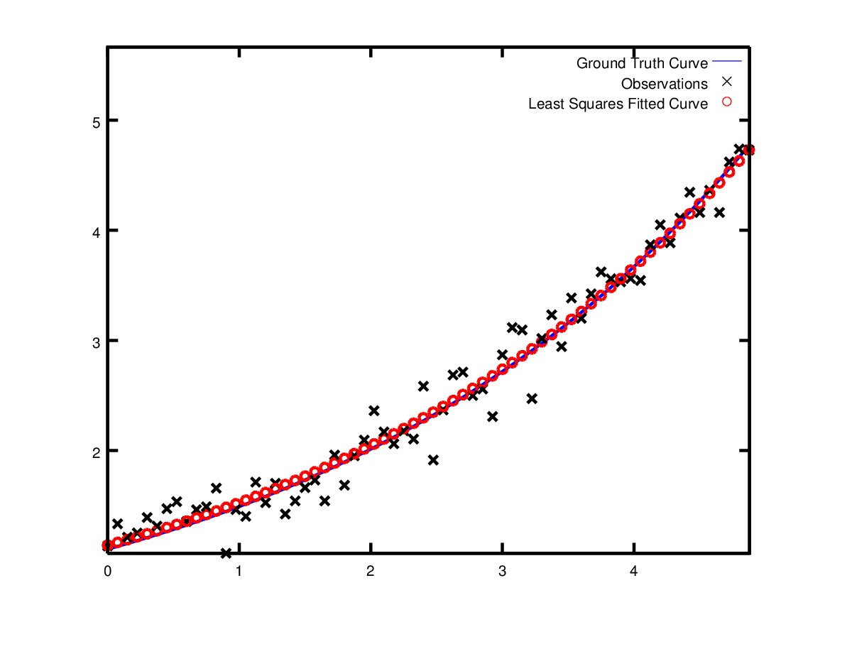
之前的例子都是不依赖数据的简单例子。非线性最小二乘法分析最初的目标是把数据拟合称曲线。现在考虑曲线拟合的数据，公式为\(y = e^{0.3x + 0.1}\)。对其进行采样并加入方差为\(\sigma = 0.2\)高斯噪声。我们希望拟合曲线
\[ y = e^{mx + c} \]
首先我们定义一个模板对象来评估残差。

struct ExponentialResidual {ExponentialResidual(double x, double y): x_(x), y_(y) {}template <typename T>bool operator()(const T* const m, const T* const c, T* residual) const {residual[0] = T(y_) - exp(m[0] * T(x_) + c[0]);return true;}private:// Observations for a sample.const double x_;const double y_;
};

假设我们有观测数据\(2n\)大小，构建如下问题。

double m = 0.0;
double c = 0.0;Problem problem;
for (int i = 0; i < kNumObservations; ++i) {CostFunction* cost_function =new AutoDiffCostFunction<ExponentialResidual, 1, 1, 1>(new ExponentialResidual(data[2 * i], data[2 * i + 1]));problem.AddResidualBlock(cost_function, NULL, &m, &c);
}

变异运行examples/curve_fitting.cc得到相应结果。

iter      cost      cost_change  |gradient|   |step|    tr_ratio  tr_radius  ls_iter  iter_time  total_time0  1.211734e+02    0.00e+00    3.61e+02   0.00e+00   0.00e+00  1.00e+04       0    5.34e-04    2.56e-031  1.211734e+02   -2.21e+03    0.00e+00   7.52e-01  -1.87e+01  5.00e+03       1    4.29e-05    3.25e-032  1.211734e+02   -2.21e+03    0.00e+00   7.51e-01  -1.86e+01  1.25e+03       1    1.10e-05    3.28e-033  1.211734e+02   -2.19e+03    0.00e+00   7.48e-01  -1.85e+01  1.56e+02       1    1.41e-05    3.31e-034  1.211734e+02   -2.02e+03    0.00e+00   7.22e-01  -1.70e+01  9.77e+00       1    1.00e-05    3.34e-035  1.211734e+02   -7.34e+02    0.00e+00   5.78e-01  -6.32e+00  3.05e-01       1    1.00e-05    3.36e-036  3.306595e+01    8.81e+01    4.10e+02   3.18e-01   1.37e+00  9.16e-01       1    2.79e-05    3.41e-037  6.426770e+00    2.66e+01    1.81e+02   1.29e-01   1.10e+00  2.75e+00       1    2.10e-05    3.45e-038  3.344546e+00    3.08e+00    5.51e+01   3.05e-02   1.03e+00  8.24e+00       1    2.10e-05    3.48e-039  1.987485e+00    1.36e+00    2.33e+01   8.87e-02   9.94e-01  2.47e+01       1    2.10e-05    3.52e-0310  1.211585e+00    7.76e-01    8.22e+00   1.05e-01   9.89e-01  7.42e+01       1    2.10e-05    3.56e-0311  1.063265e+00    1.48e-01    1.44e+00   6.06e-02   9.97e-01  2.22e+02       1    2.60e-05    3.61e-0312  1.056795e+00    6.47e-03    1.18e-01   1.47e-02   1.00e+00  6.67e+02       1    2.10e-05    3.64e-0313  1.056751e+00    4.39e-05    3.79e-03   1.28e-03   1.00e+00  2.00e+03       1    2.10e-05    3.68e-03
Ceres Solver Report: Iterations: 13, Initial cost: 1.211734e+02, Final cost: 1.056751e+00, Termination: CONVERGENCE
Initial m: 0 c: 0
Final   m: 0.291861 c: 0.131439

使用初值\(m=0, c=0\), 初始目标函数值为\(121.173\)。Ceres计算得到\(m=0.291, c=0.131\).目标函数值为\(1.056\)。但这同原始模型不一样，但也是合理的。通过带噪声的数据恢复模型会得到一定的偏差。实际上，即使使用原始模型数据，偏差更大。

实战之曲线鲁棒拟合

现在假设数据有一些我们并不在模型的值。如果使用这些做拟合，模型会离真实值有所偏差。如下图。

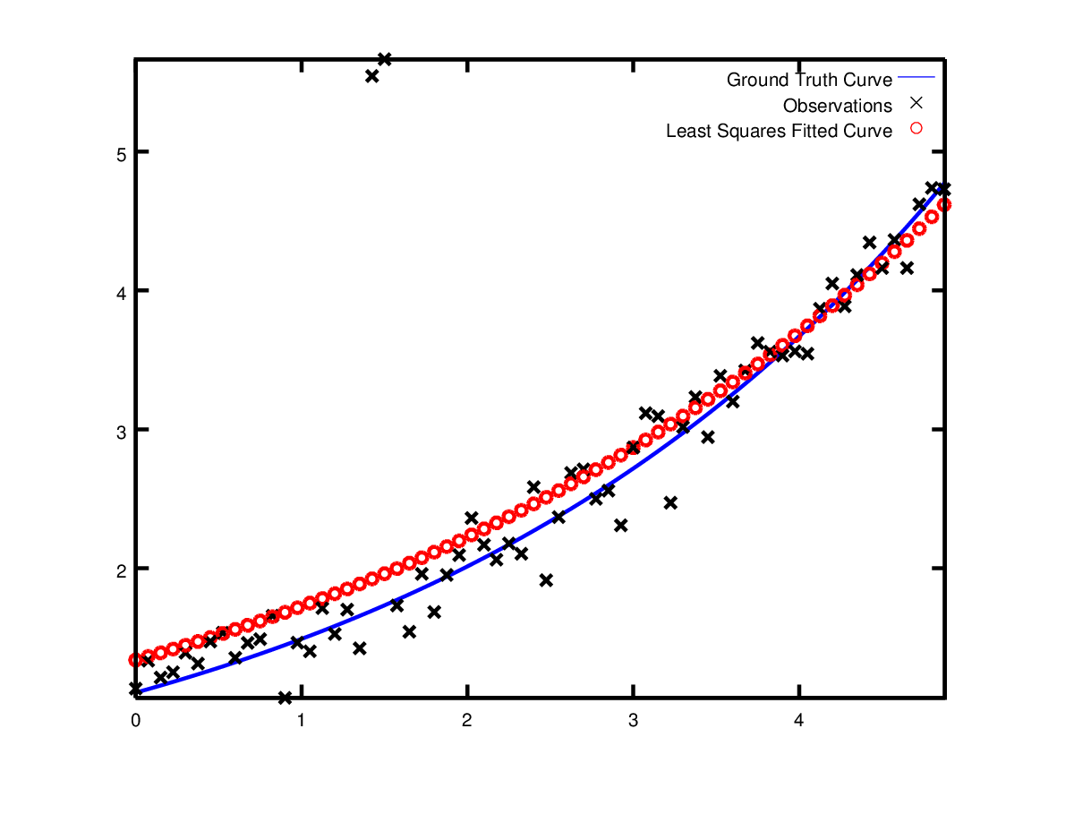
为了处理这些噪点，一个技巧是使用LossFunction。此函数减小大偏差对整个残差模块的影响。大偏差经常属于Outliers。加入残差函数，我们修要做修改

problem.AddResidualBlock(cost_function, NULL , &m, &c);

改为

problem.AddResidualBlock(cost_function, new CauchyLoss(0.5) , &m, &c);

CauchyLoss是Ceres Solver发明的损失函数之一。0.5是损失函数的尺度。加入损失函数后，我们获得更好的拟合结果。

下一篇文章里，我们重点介绍Ceres是计算机三维视觉里的重要应用：光束平差法（Bundle Adjustment），一般简称BA。