sql server 入门_SQL Server中的数据挖掘入门

sql server 入门

介绍 (Introduction)

In past chats, we have had a look at a myriad of different Business Intelligence techniques that one can utilize to turn data into information. In today’s get together we are going to have a look at a technique dear to my heart and often overlooked. We are going to be looking at data mining with SQL Server, from soup to nuts.

在过去的聊天中，我们了解了无数种可以用来将数据转换为信息的不同商业智能技术。在今天的聚会中，我们将了解一种我心中常常被忽视的技术。我们将研究使用SQL Server进行数据挖掘的过程，从无所不包。

Microsoft has come up with a fantastic set of data mining tools which are often underutilized by Business Intelligence folks, not because they are of poor quality but rather because not many folks know of their existence OR due to the fact that people have never had to opportunity to get to utilize them.

微软提供了一套出色的数据挖掘工具，这些工具经常被商业情报人员利用，这不是因为它们的质量很差，而是因为没有多少人知道他们的存在，或者是因为人们从来没有机会去利用它们。

Rest assured that you are NOW going to get a bird’s eye view of the power of the mining algorithms in our ‘fire-side’ chat today.

请放心，您现在将在今天的“火边”聊天中大致了解挖掘算法的功能。

As I wish to describe the “getting started” process in detail, this article has been split into two parts. The first describes exactly this (getting started), whilst the second part will discuss turning the data into real information.

正如我希望详细描述“入门”过程一样，本文分为两部分。第一部分准确地描述了这一点（入门），而第二部分将讨论将数据转换为真实信息。

So ‘grab a pick and shovel’ and let us get to it!

因此，“抢一把铲子”，让我们开始吧！

入门 ( Getting started )

For today’s exercise, we start by having a quick look at our source data. It is a simple relational table within the SQLShackFinancial database that we have utilized in past exercises.

对于今天的练习，我们首先快速查看源数据。它是我们在过去的练习中使用SQLShackFinancial数据库中的简单关系表。

As a disclosure, I have changed the names and addresses of the true customers for the “production data” that we shall be utilizing. The names and addresses of the folks that we shall utilize come from the Microsoft Contoso database. Further, I have split the client data into two distinct tables: one containing customer numbers under 25000 and the other with customer numbers greater than 25000. The reason for doing so will become clear as we progress.

作为披露，我更改了我们将要使用的“生产数据”的真实客户的名称和地址。我们将利用的人员的姓名和地址来自Microsoft Contoso数据库。此外，我已经将客户数据分为两个不同的表：一个包含25000以下的客户编号，另一个包含大于25000的客户编号。这样做的原因将随着我们的发展而变得清楚。

Having a quick look at the customer table (containing customer numbers less than 25000), we find the following data.

快速浏览客户表（包含少于25000的客户号），我们发现以下数据。

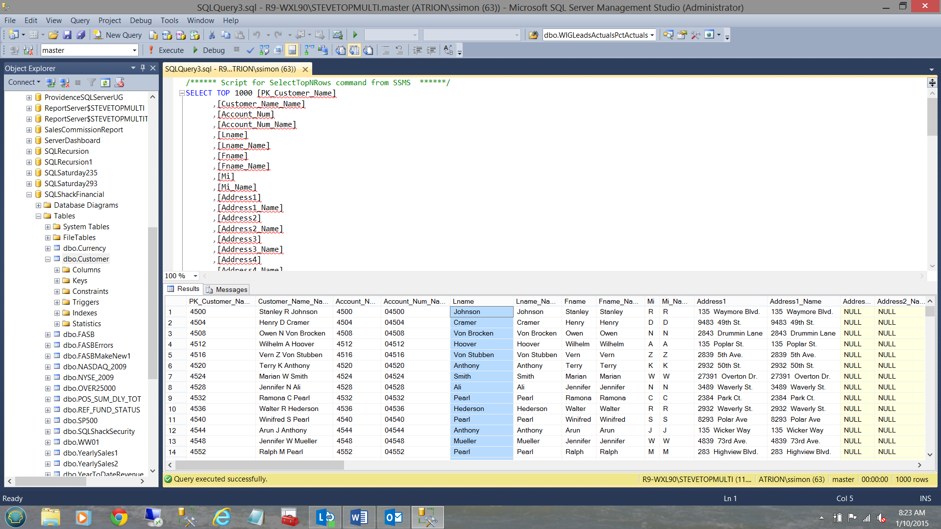
The screenshot above shows the residential addresses of people who have applied for financial loans from SQLShack Finance.

上面的屏幕截图显示了从SQLShack Finance申请了金融贷款的人的住所。

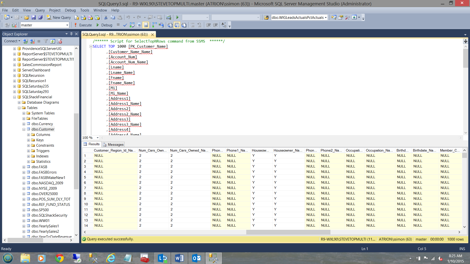
Moreover, the data shows criteria such as the number of cars that the applicant owns, his or her marital status and whether or not he or she owns a house. NOTE that I have not mentioned the person’s income or net worth. This is will come into play going forward.

此外，数据还显示一些标准，例如申请人拥有的汽车数量，他或她的婚姻状况以及他或她是否拥有房屋。注意，我没有提及该人的收入或净资产。这将在未来发挥作用。

创建我们的采矿项目 ( Creating our mining project )

Now that we have had a quick look at our raw data, we open SQL Server Data Tools (henceforward referred to as SSDT) to begin our adventure into the “wonderful world of data mining”.

现在，我们已经快速浏览了原始数据，我们将打开SQL Server数据工具（以下称为SSDT）开始我们的冒险，进入“精彩的数据挖掘世界”。

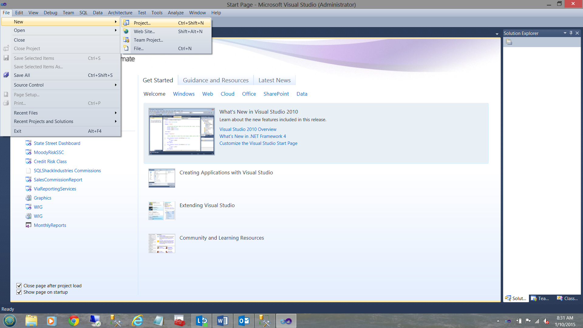
Opening SSDT, we select “New” from the “File” tab on the activity ribbon and select “Project” (see above).

打开SSDT，我们从活动功能区的“文件”选项卡中选择“新建”，然后选择“项目”（见上文）。

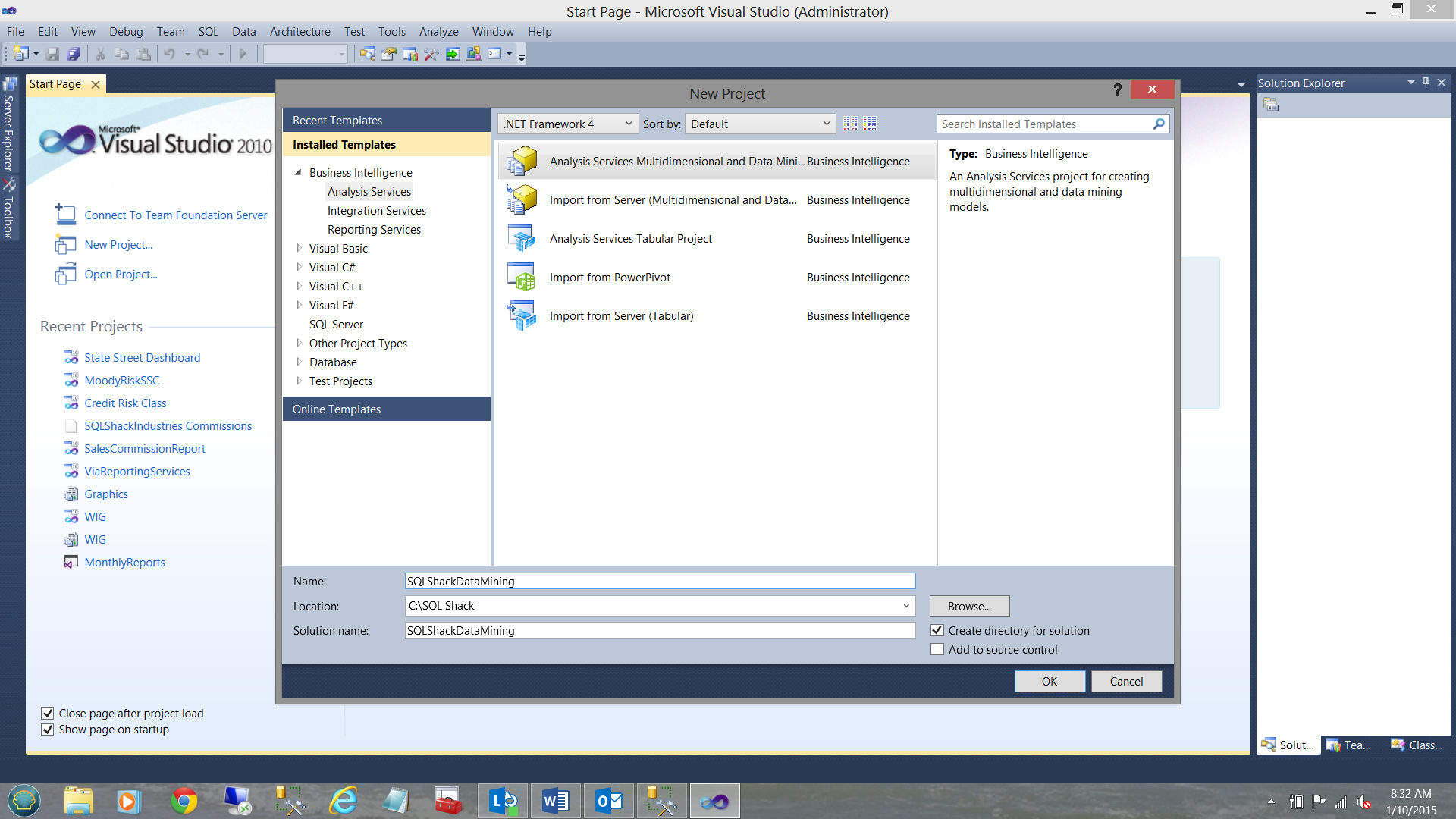
We select the “Analysis Services Multidimensional and Data Mining” option. We give our new project a name and click OK to continue.

我们选择“ Analysis Services多维和数据挖掘”选项。我们给新项目起一个名字，然后单击“确定”继续。

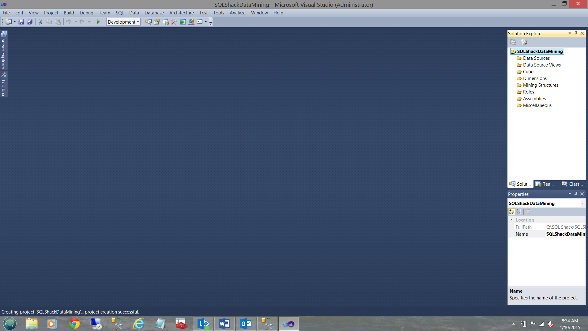
Having clicked “OK”, we find ourselves on our working surface.

单击“确定”后，我们发现自己在工作表面上。

Our first task is to establish a connection to our relational data. We do this by creating a new “Data Source” (see below).

我们的首要任务是建立与我们的关系数据的连接。为此，我们创建了一个新的“数据源”（见下文）。

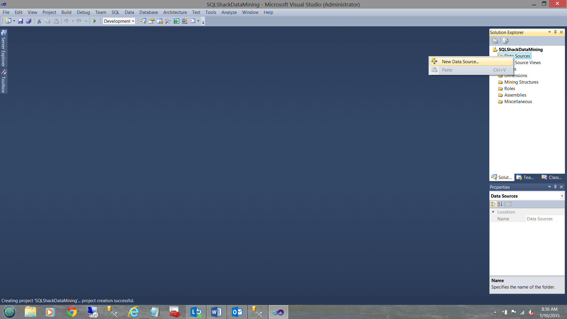
We right-click on the “Data Sources” folder (see above and to the right) and select the “New Data Source” option.

我们右键单击“数据源”文件夹（请参见上方和右侧），然后选择“新数据源”选项。

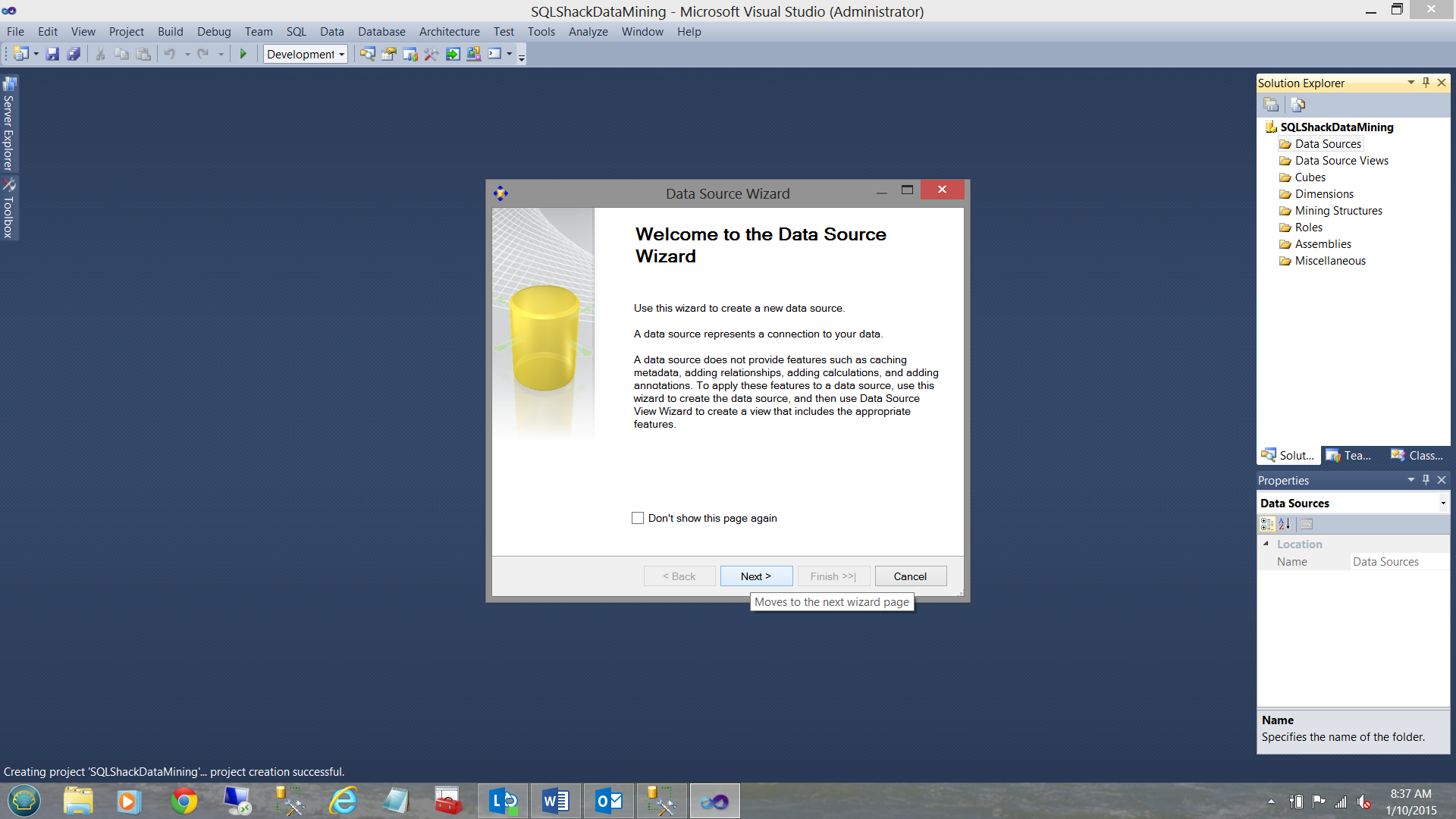
The “New Data Source” Wizard is brought up. We click “Next”.

出现“新数据源”向导。我们点击“下一步”。

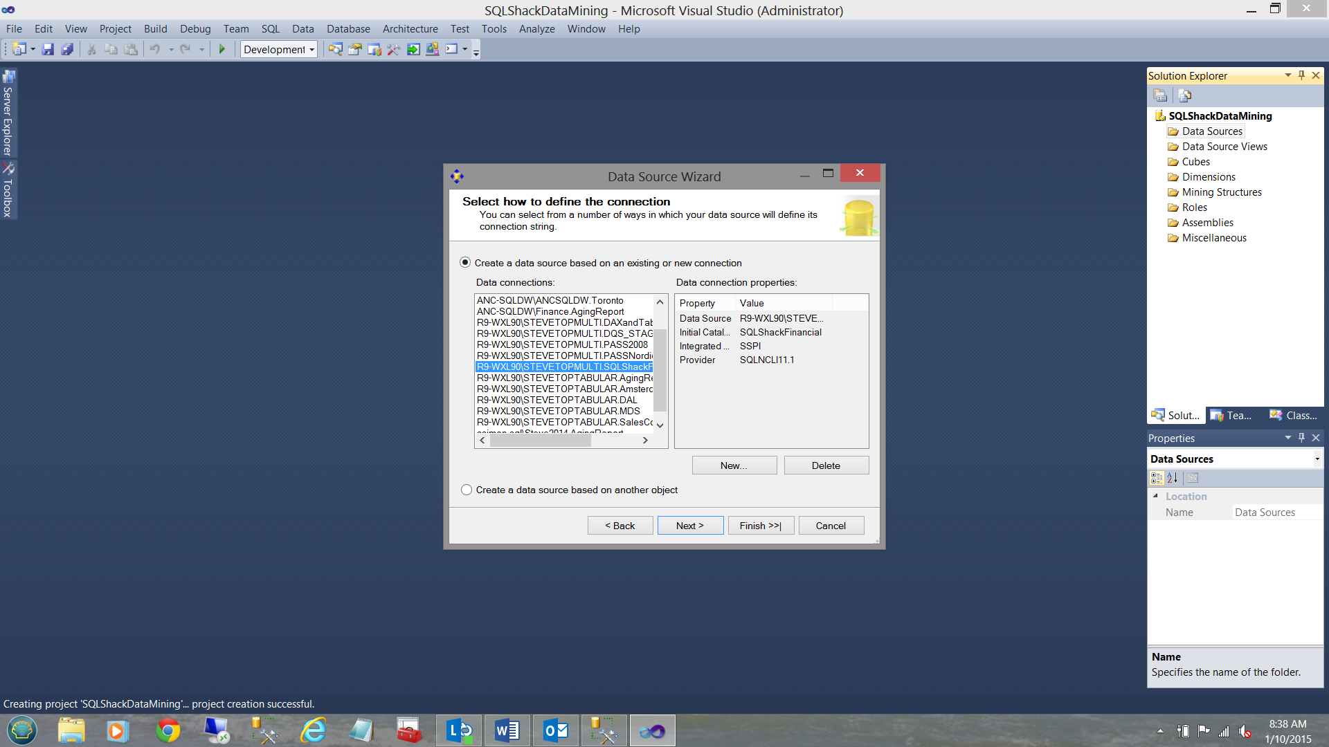
We now find ourselves looking at connections that we have used in past and SSDT wishes to know which (if any) of these connections we wish to utilize. We choose our “SQLShackFinancial” connection.

现在，我们发现自己正在查看过去使用的连接，SSDT希望知道我们希望使用这些连接中的哪些（如果有）。我们选择“ SQLShackFinancial”连接。

We select “Next”

我们选择“下一步”

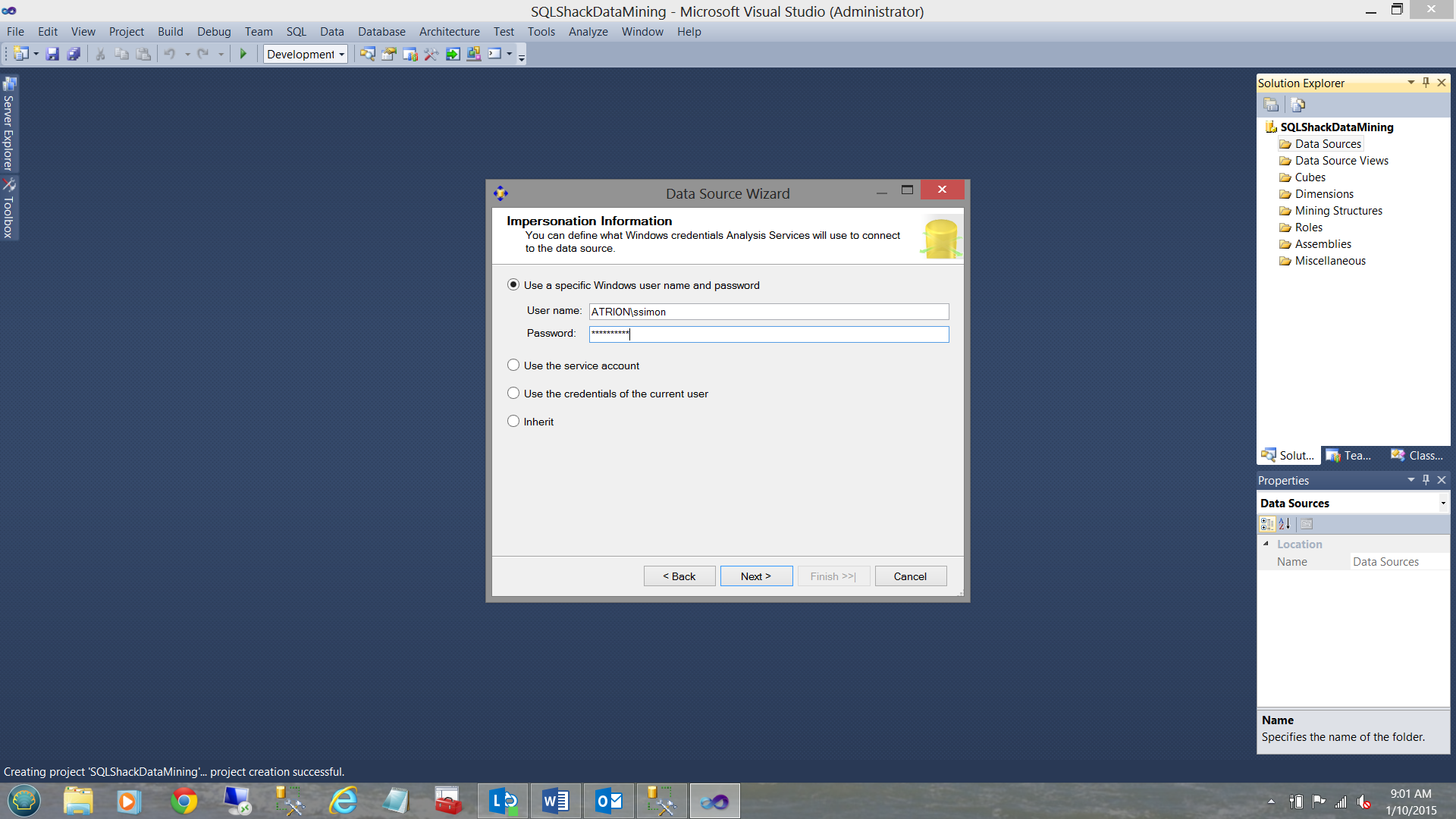
We are asked for our credentials (see above) and click next.

要求我们提供凭据（见上文），然后单击下一步。

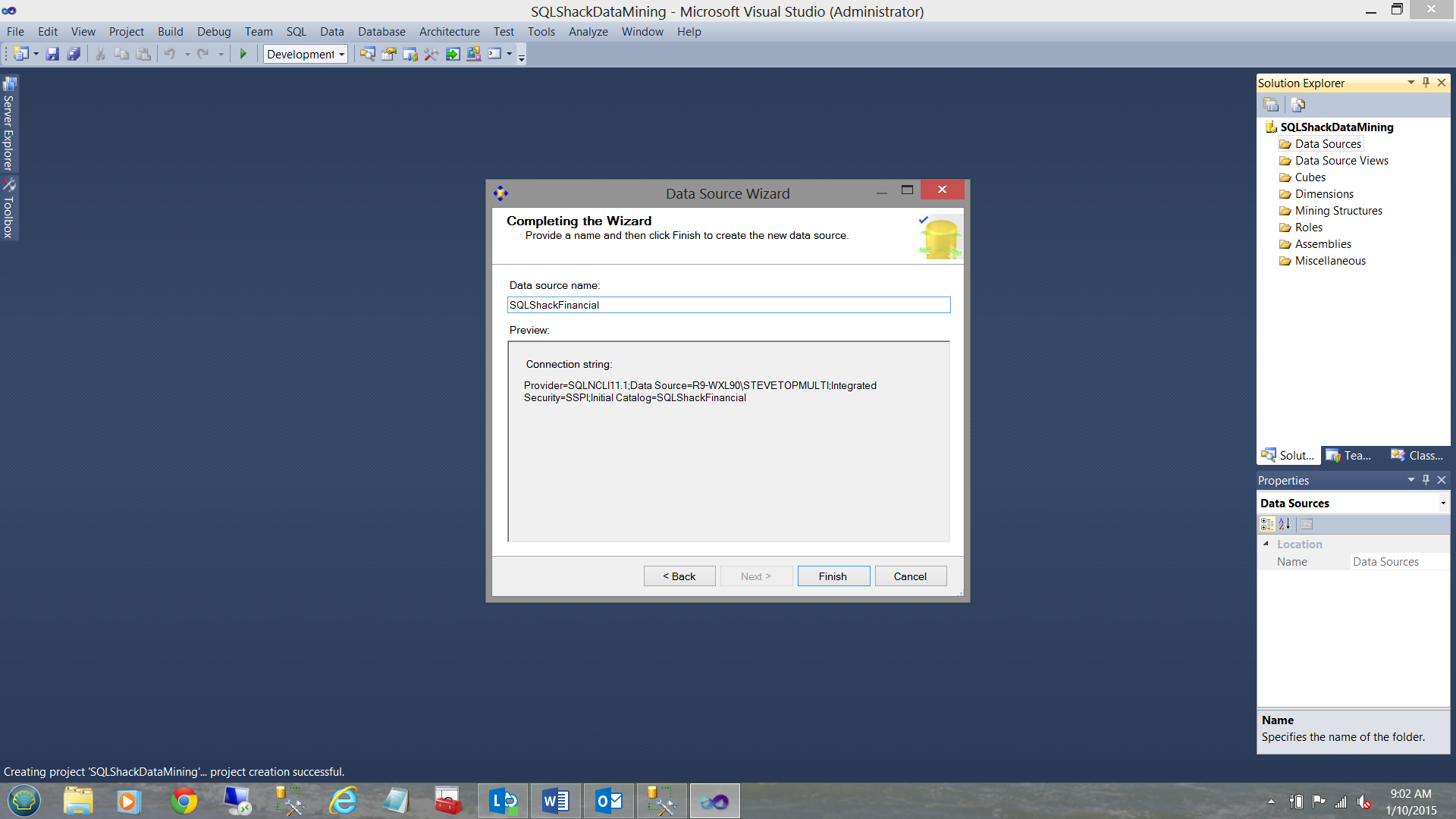
We are now asked to give a name to our connection (see above).

现在，我们被要求给我们的连接起一个名字（见上文）。

We click finish.

我们点击完成。

创建我们的数据源视图 ( Creating our Data Source View )

Our next task is to create a Data Source View. This is different to what we have done in past exercises.

我们的下一个任务是创建一个数据源视图。这与我们在过去的练习中所做的不同。

The data source view permits us to create relationships (from our relational data) which we wish to carry forward into the ‘analytic world’. One may think of a “Data Source View” as a staging area for our relational data prior to its importation into our cubes and mining models.

数据源视图使我们能够（希望从关系数据中）创建关系，并希望将这些关系推向“分析世界”。在将关系数据导入多维数据集和挖掘模型之前，可以将“数据源视图”视为关系数据的暂存区域。

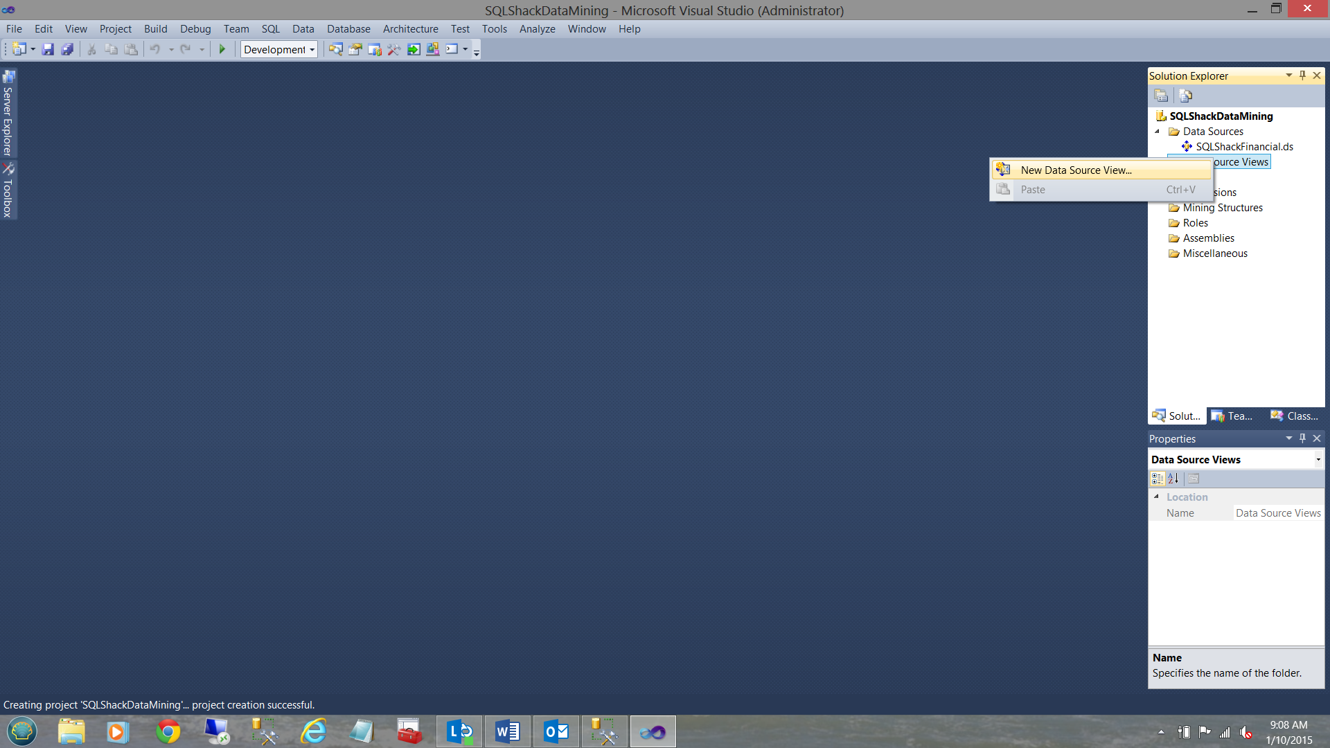
We right-click on the “Data Source Views” folder and select “New Data Source View”.

我们右键单击“数据源视图”文件夹，然后选择“新数据源视图”。

The “Data Source View” wizard is brought up (see below).

出现“数据源视图”向导（请参见下文）。

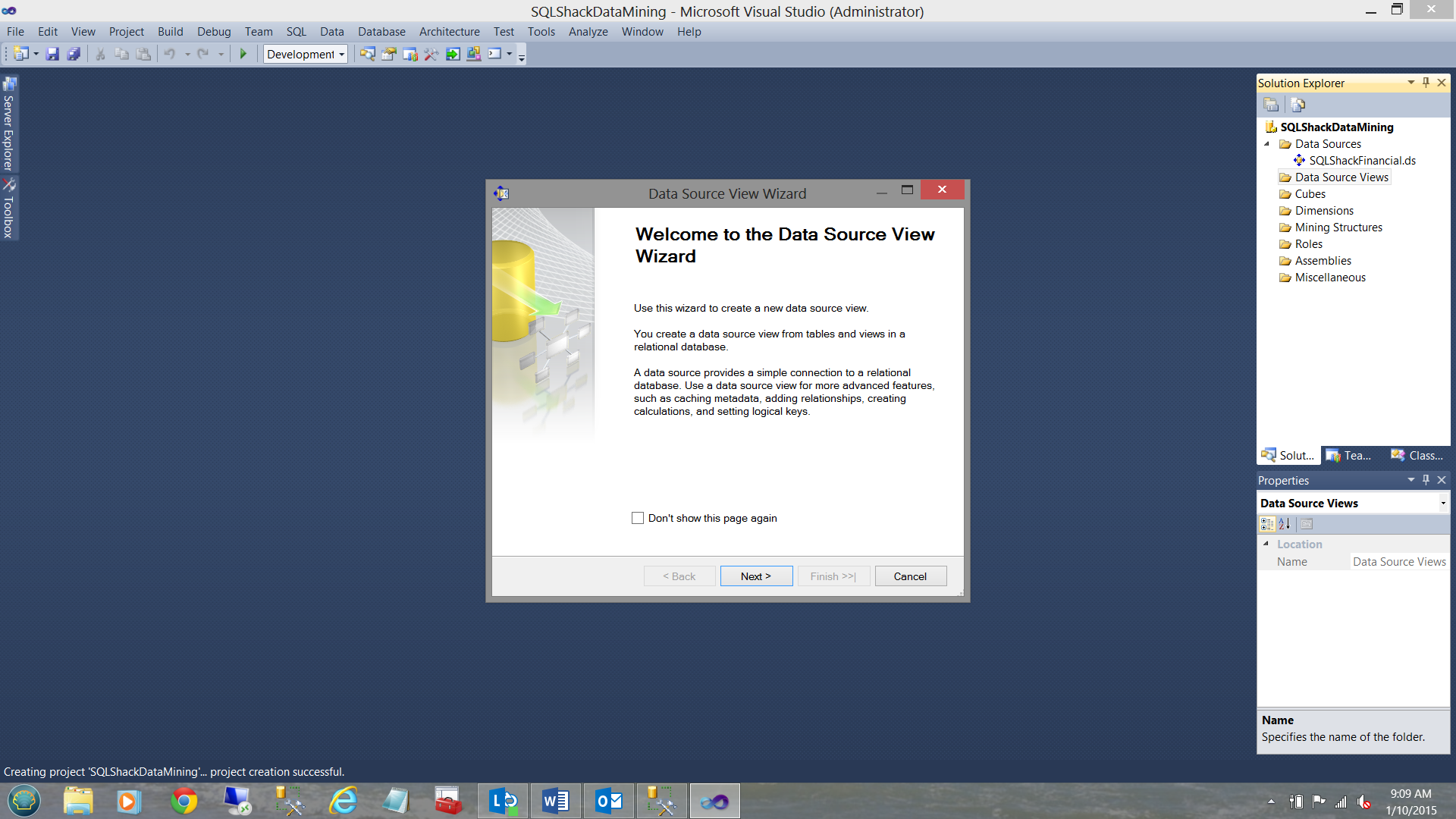
We click “Next” (see above).

我们单击“下一步”（见上文）。

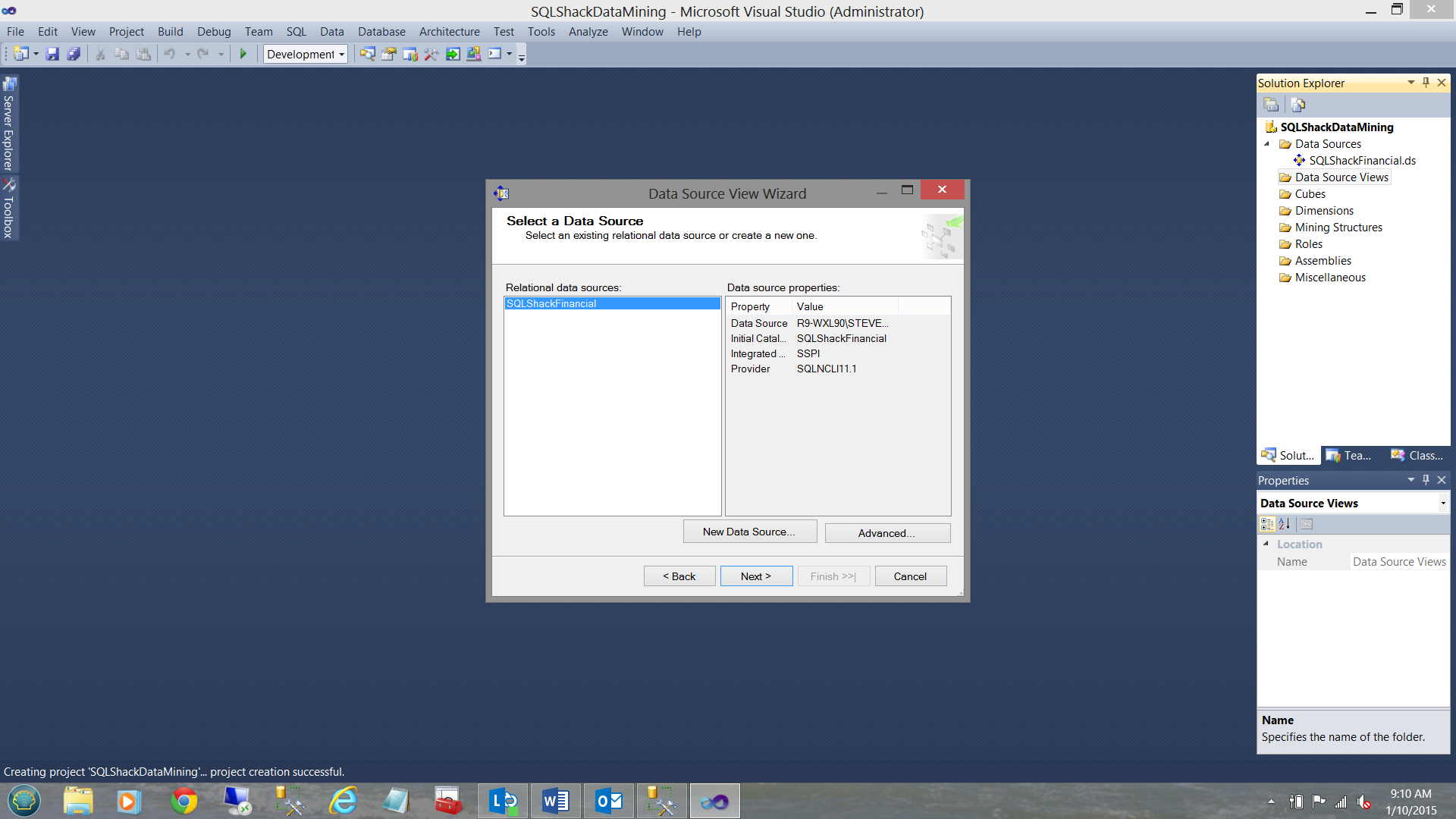
We select our “Data Source” that we defined above (see above).

我们选择上面定义的“数据源”（请参见上文）。

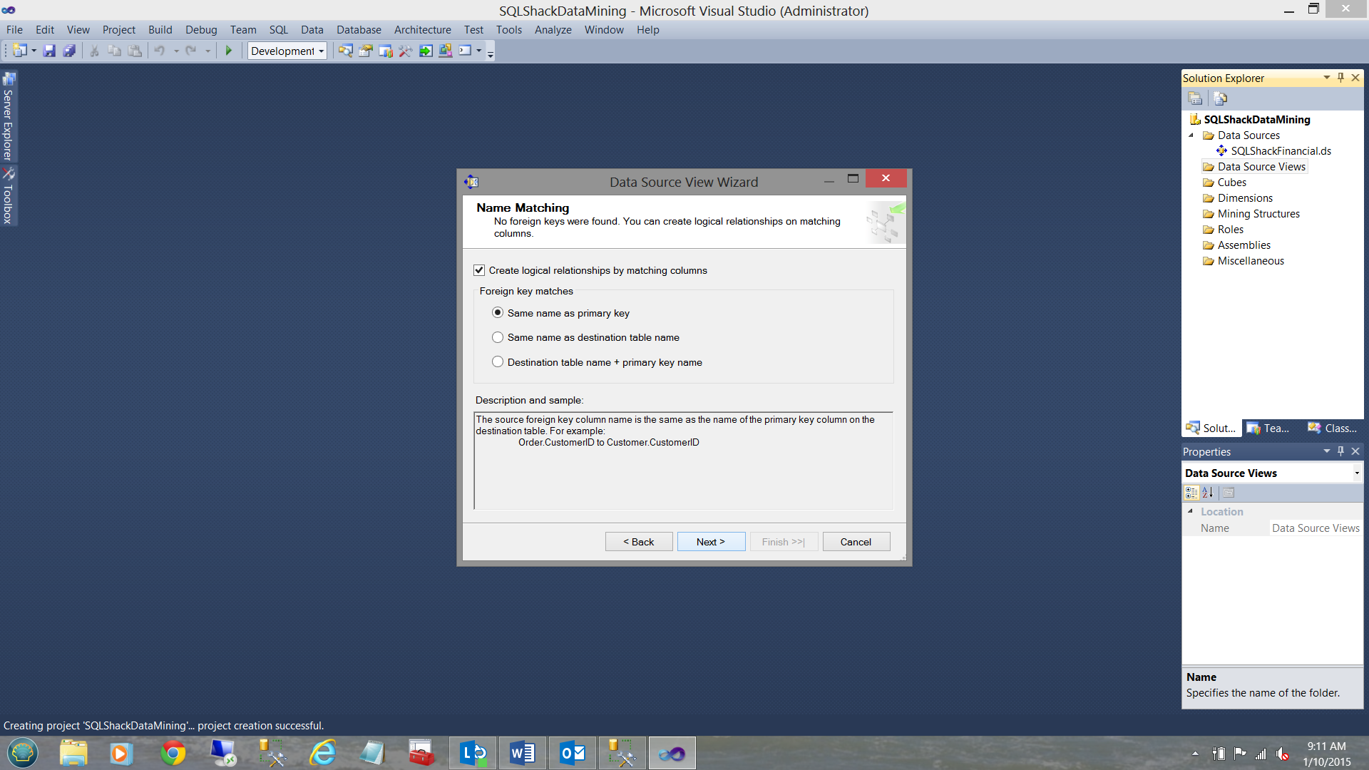
The “Name Matching” dialogue box is brought into view. As we shall be working with one table for this exercise, there is not much impact from this screen HOWEVER if we were creating a relationship between two or more tables we would indicate to the system that we want it to create the necessary logical relationships between the two or more tables to ensure that our tables are correctly joined.

出现“名称匹配”对话框。由于我们将使用一个表进行此练习，因此，如果在两个或多个表之间创建关系，则此屏幕不会产生太大影响，但会向系统指示我们希望系统在表之间创建必要的逻辑关系。两个或更多表，以确保我们的表正确连接。

In our case we merely select “Next” (see above).

在我们的情况下，我们仅选择“下一步”（请参见上文）。

We are now asked to select the table or tables that we wish to utilize.

现在，要求我们选择希望使用的一个或多个表。

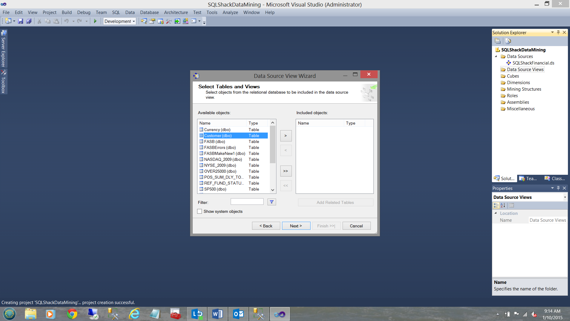
For our current exercise, I select the “Customer” table (See above) and move the table to the “Included Objects” (see below).

对于我们当前的练习，我选择“客户”表（见上文），然后将该表移至“包含的对象”（见下文）。

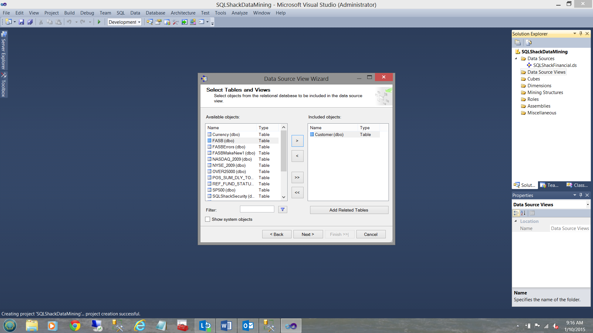
We then click “Next”.

然后，我们单击“下一步”。

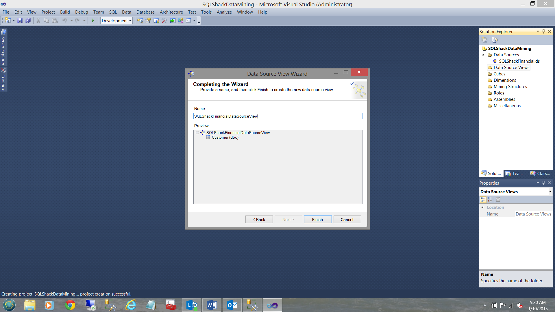
We are now asked to give our “Data Source View” a name (see above) and we then click “Finish” to complete this task.

现在，我们要求给“数据源视图”命名（请参见上文），然后单击“完成”以完成此任务。

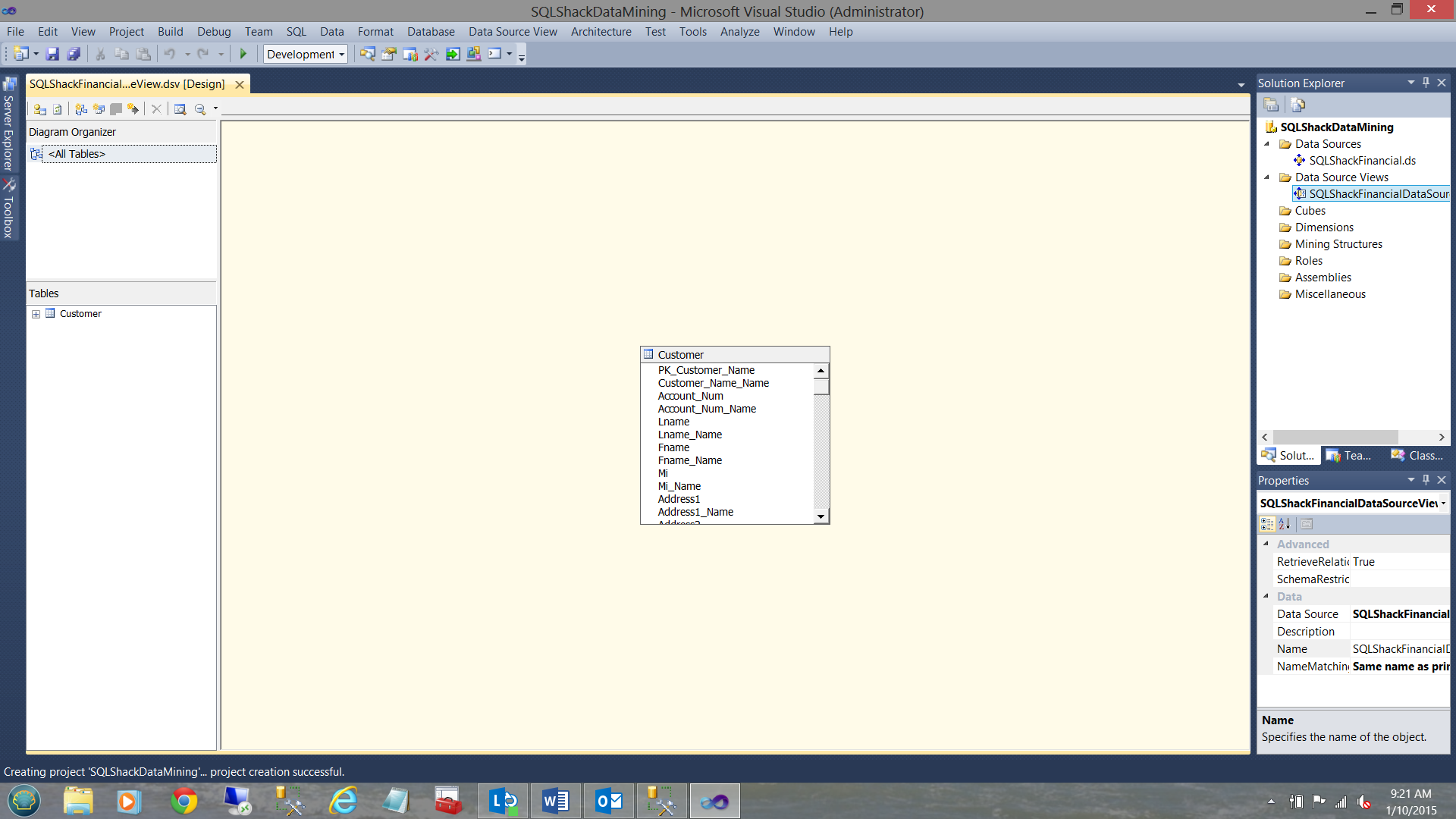
We find ourselves back on our work surface. Note that the Customer entity is now showing in the center of the screenshot above, as is the name of the “Data Source View” (see upper right).

我们发现自己回到了工作现场。请注意，Customer实体现在显示在上方屏幕快照的中心，“数据源视图”的名称也是如此（请参见右上方）。

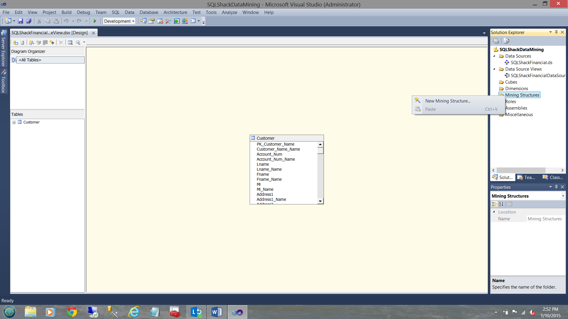
We now right click on the ‘Mining Structure” folder and select “New Mining Structure” (see above).

现在，我们右键单击“ Mining Structure”文件夹，然后选择“ New Mining Structure”（请参见上文）。

The “Data Mining Wizard” now appears (see below).

现在出现“数据挖掘向导”（见下文）。

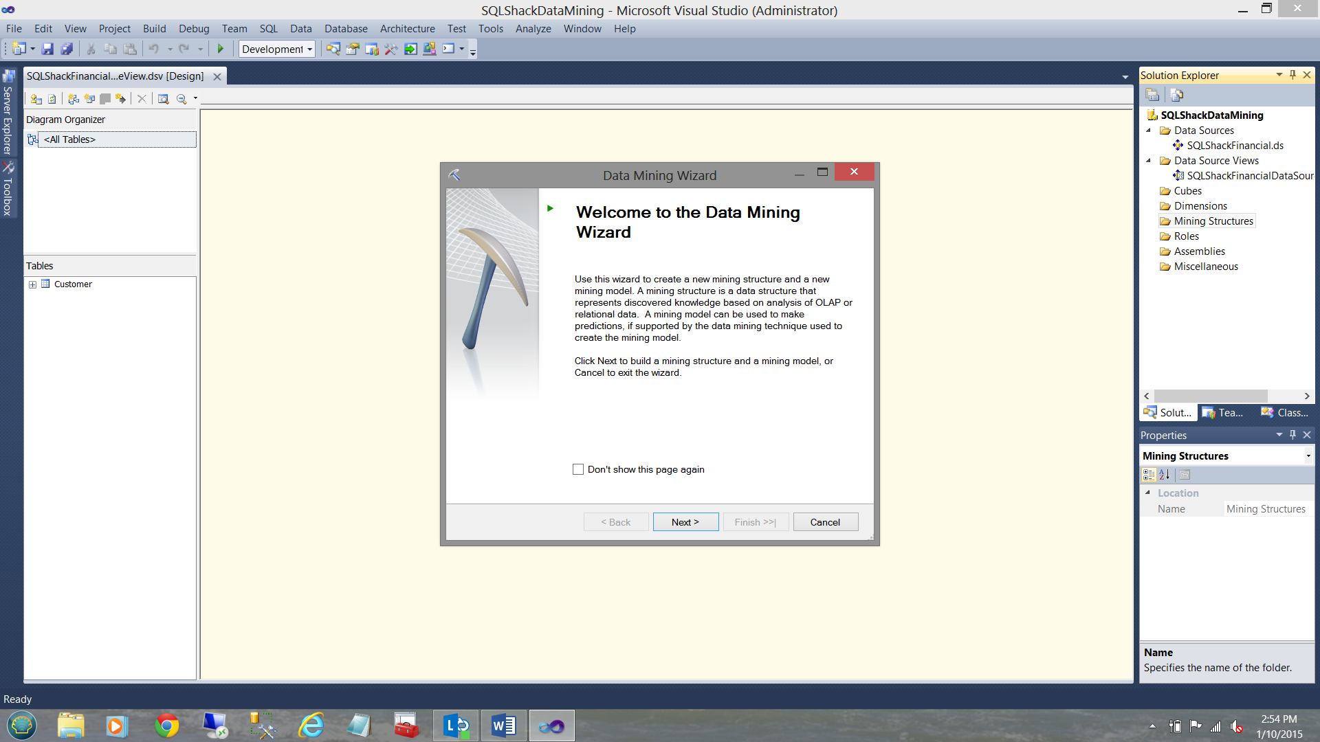
We click “Next”.

我们点击“下一步”。

For the “Select the Definition Method” screen we shall accept the default “From existing relational database or data warehouse” option (see below).

对于“选择定义方法”屏幕，我们将接受默认的“来自现有关系数据库或数据仓库”选项（请参见下文）。

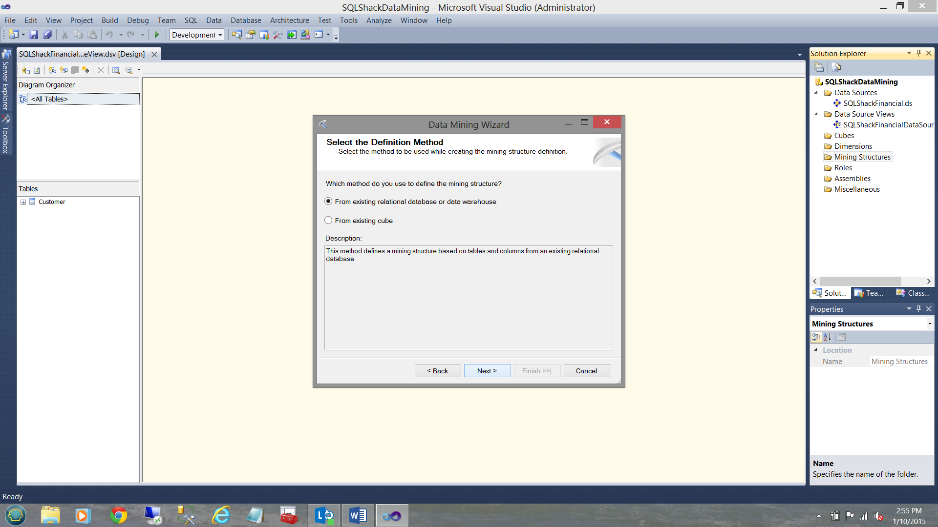
We then click “Next”.

然后，我们单击“下一步”。

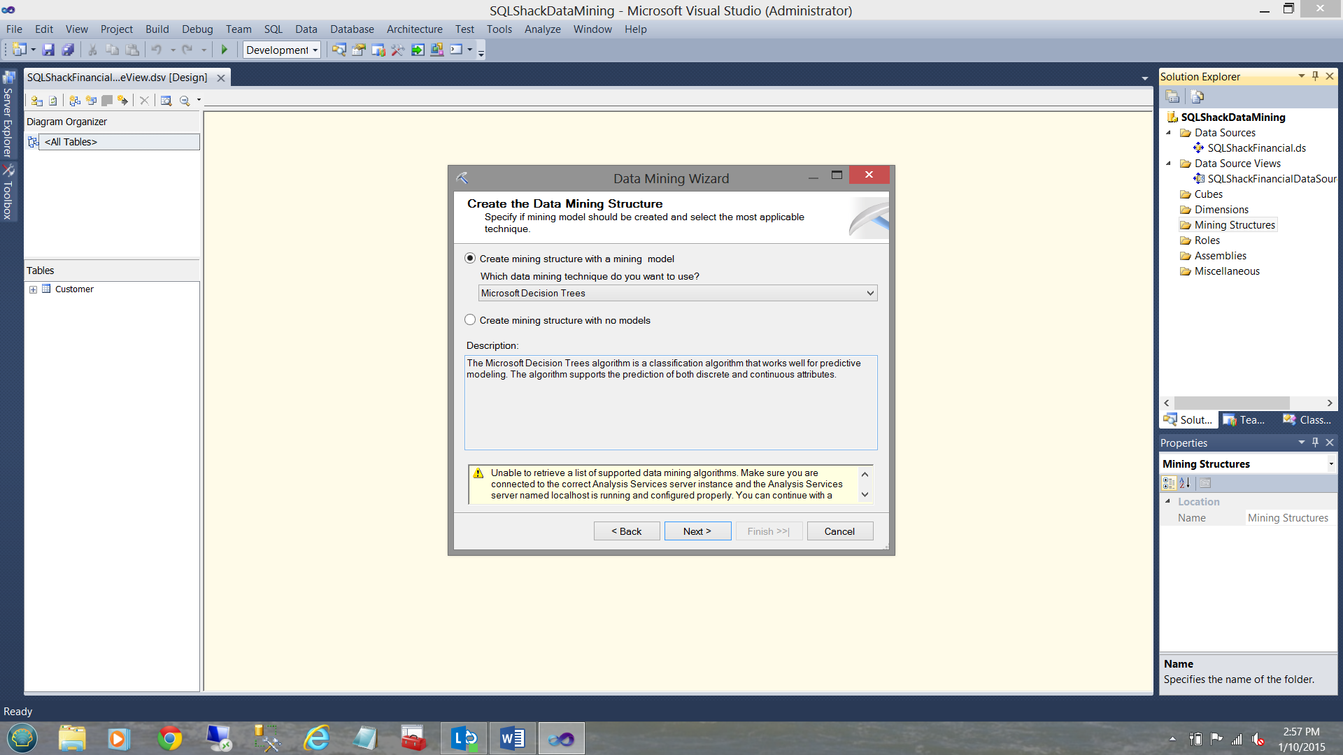
The “Create the Data Mining Structure” screen is brought into view. The wizard asks us which mining technique we wish to use. In total for this exercise, we shall be creating four structure. “Microsoft Decision Trees” is one of the four. That said, we shall leave the default setting “Microsoft Decision Trees” as is.

进入“创建数据挖掘结构”屏幕。向导将询问我们希望使用哪种挖掘技术。总的来说，我们将创建四个结构。 “ Microsoft决策树”是这四个之一。也就是说，我们将保留默认设置“ Microsoft Decision Trees”。

We ignore the warning shown in the message box as we shall create the necessary connectivity on the next few screens.

我们将忽略消息框中显示的警告，因为我们将在接下来的几个屏幕上创建必要的连接。

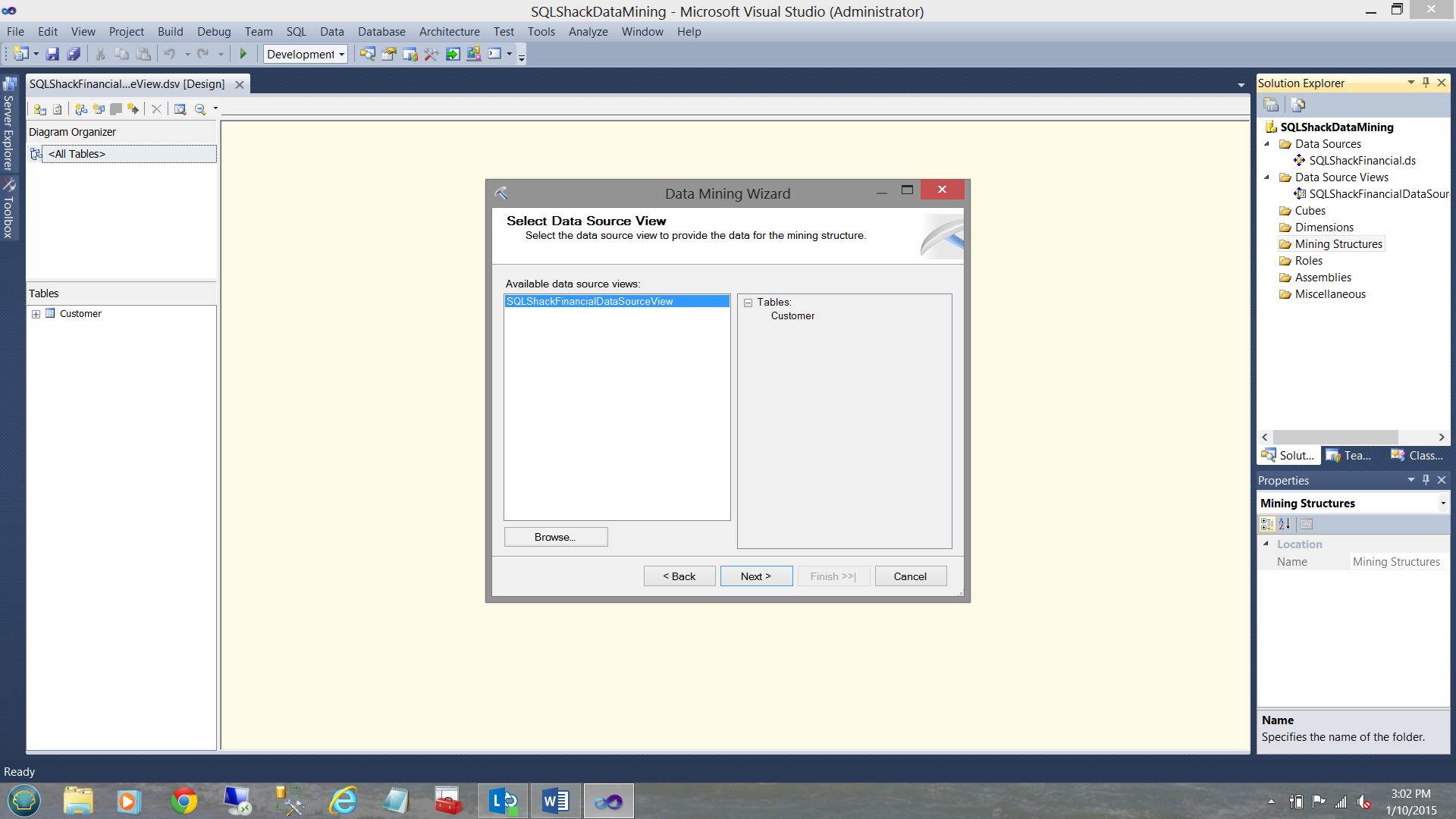
The reader will note that the system wishes to know which “Data Source View” we wish to utilize. We select the one that we created above. We then click “Next”.

读者会注意到，该系统希望知道我们希望使用哪种“数据源视图”。我们选择上面创建的那个。然后，我们单击“下一步”。

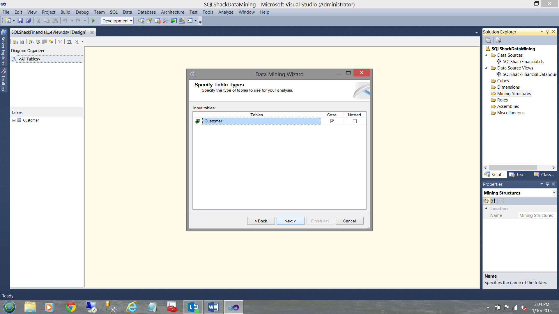
The mining wizard now asks us to let it know where the source data resides. We select the “Customer” table (see above) and we click next.

现在，挖掘向导会要求我们告知源数据所在的位置。我们选择“客户”表（见上文），然后单击下一步。

At this point, we need to understand that once the model is created we shall “process” the model. Processing the model achieves two important things. First it “Trains” the model as to what type of data we are utilizing and runs that data against the data mining model that we have selected. After obtaining the necessary results, the process compares the actual results with the predicted results. The closer the actuals are to the predicted results the more accurate the model that we selected. The reader should note that whilst Microsoft provides us with +/- twelve mining models NOT ALL will provide a satisfactory solution and therefore a different model may need to be used. We shall see just this within a few minutes.

在这一点上，我们需要了解，一旦创建了模型，我们将“处理”该模型。处理模型可以实现两件重要的事情。首先，它“训练”该模型以了解我们正在使用什么类型的数据，并根据我们选择的数据挖掘模型来运行该数据。在获得必要的结果后，该过程会将实际结果与预测结果进行比较。实际值与预测结果越接近，我们选择的模型越准确。读者应注意，尽管Microsoft为我们提供了+/-十二种采矿模型，但并非ALL会提供令人满意的解决方案，因此可能需要使用其他模型。我们将在几分钟内看到这一点。

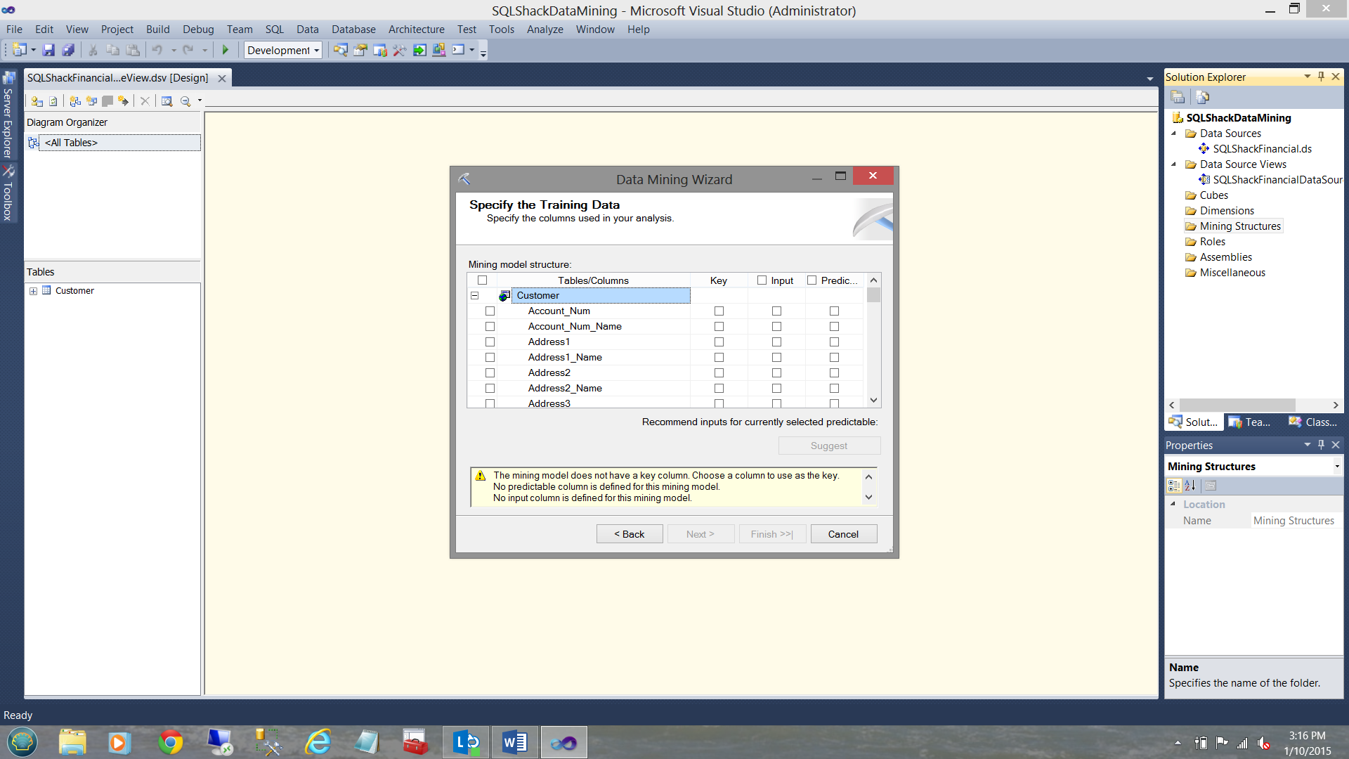
We now must specify the “training data” or in simple terms “introduce the Microsoft mining models to the customer raw data and see what the mining model detects”. In our case, it is the data from the “Customer” table. What we must do is to provide the system with a Primary Key field. Further, we must tell the system what data fields/criteria will be the data inputs that will be utilized with the mining model to see what correlation (if any) there is between these input fields (Does the client owns a house? How many cars does the person own? Is he or she married?) and what we wish to ascertain from the “Predicted” field (Is the person a good credit risk?) .

现在，我们必须指定“训练数据”或简单地说“将Microsoft挖掘模型引入客户原始数据并查看挖掘模型检测到的内容”。在我们的例子中，它是“客户”表中的数据。我们必须做的是为系统提供主键字段。此外，我们必须告诉系统哪些数据字段 / 条件将是挖掘模型将使用的数据输入，以查看这些输入字段之间存在什么关联（如果有）（客户是否拥有房屋？有多少辆汽车？该人拥有吗？是否已婚？）以及我们希望从“预测”字段中确定的内容（该人是否存在良好的信用风险？）。

设置主键 ( Setting the Primary Key )

For the primary key we select the fields “PK_Customer_Name” (see above).

对于主键，我们选择“ PK_Customer_Name”字段（请参见上文）。

选择输入参数/字段 ( Selecting the input parameters / fields )

We select “Houseowner” and “Marital_Status” (see above)

我们选择“房主”和“婚姻状况”（见上文）

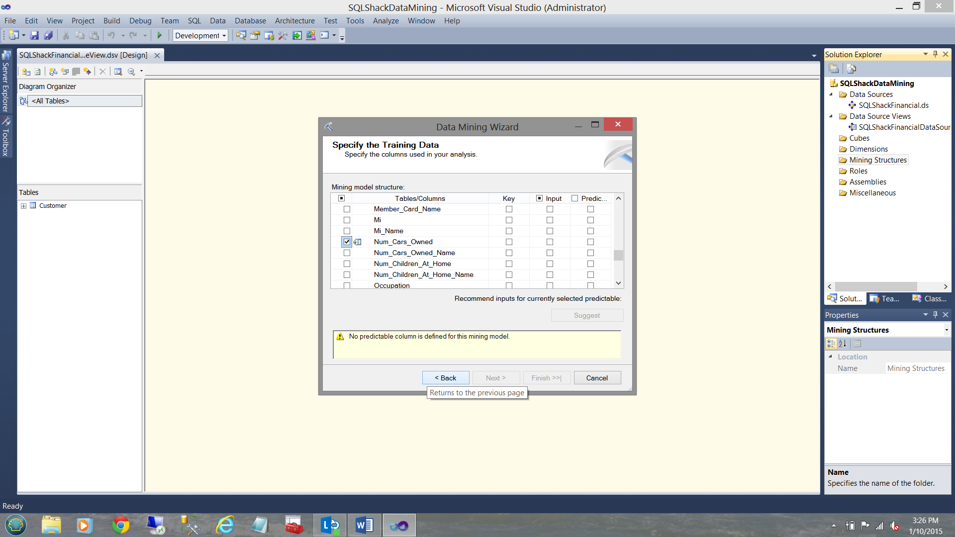
and “number of cars owned” (see above)

和“拥有的汽车数量”（见上文）

As the reader will see from the two screen shots above, we selected

读者将从上面的两个屏幕截图中看到，我们选择了

Does the applicant own a house?申请人是否拥有房屋？
Is he or she married?他或她结婚了吗？
How many cars does he / she owns.他/她拥有多少辆汽车。

NOTE that I have not included income and this was deliberate for our example.

注意，我没有包括收入，这是我们的示例所故意的。

Bernie Madoff’s income was large however we KNOW that he would not be a good risk.

伯尼·麦道夫（Bernie Madoff）的收入很大，但是我们知道他不会冒很大的风险。

Lastly, included within the raw data was a field called Credit Class which are KNOWN credit ratings for the clients concerned.

最后，原始数据中包含一个名为“信用等级”的字段，该字段是有关客户的已知信用等级。

选择PREDICTED字段 ( Selecting the PREDICTED field )

Last but not least, we must select the field that we wish the mining model to predict. This field is the “Credit Class” as may be seen below:

最后但并非最不重要的一点是，我们必须选择希望挖掘模型预测的字段。该字段是“信用等级”，如下所示：

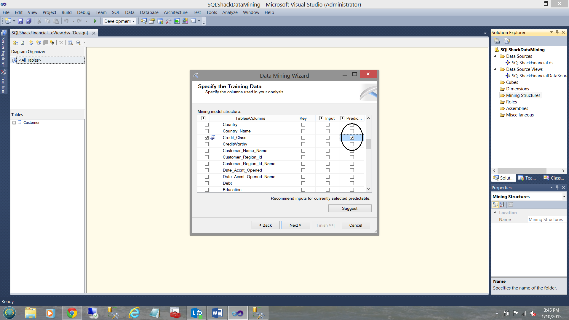
回顾一下： ( To recap: )

The primary key is “PK_Customer_name”主键是“ PK_Customer_name”
1. Is the person married?这个人结婚了吗？
2. Is the person a house owner?这个人是房主吗？
3. How many cars does the person own?该人拥有几辆车？
The field that we want the SQL Server Data Mining Algorithm to predict is the credit “bucket” that the person should fall into.. 0 being a good candidate and 4 being the worst possible candidate.我们希望SQL Server数据挖掘算法进行预测的字段是该人应该落入的信誉“桶”。0为好候选人，4为最差的候选人。

We now click “Next”.

现在，我们单击“下一步”。

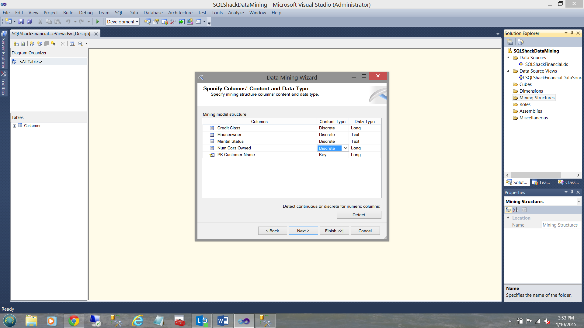
Having clicked “Next we arrive at the “Specify Columns’ Content and Data Type Screen”.

单击“下一步，我们进入”指定列的内容和数据类型屏幕”。

Credit class (the predicted field) is either a 0, 1, 2, 3, 4. These are discrete values (see above).

信用等级（预测字段）为0、1、2、3、4。这些是离散值（请参见上文）。

The number of cars owned is also a discrete value. No person owns 1.2 cars.

拥有的汽车数量也是一个离散值。没有人拥有1.2辆汽车。

House Owner is a Boolean (Y or N).

房主是布尔值（Y或N）。

Marital (Married) status is also a Boolean Value (Y or N).

婚姻（已婚）状态也是布尔值（Y或N）。

We click next.

我们点击下一步。

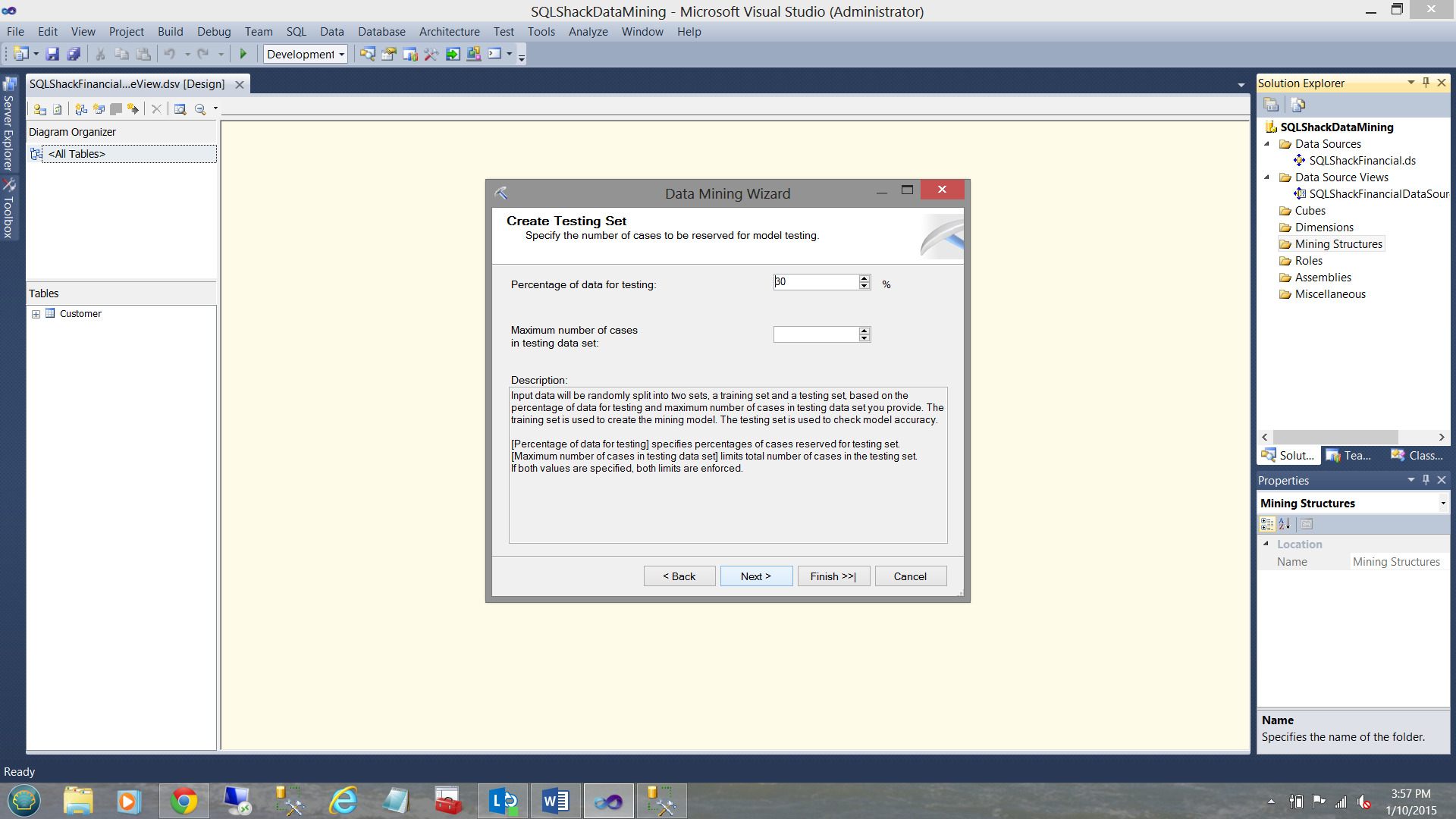
SQL Server now wishes to know of all the records within the customer table, what percentage of the data (RANDOMLY SELECTED BY THE MINING ALGORITHM) should be utilized to test just how closely the predicted values of “Credit class” tie with the actual values of “Credit Class”. One normally accept 30% as a good sample (of the population). As a reminder to the reader, the accounts within the data ALL have account numbers under 25000. We shall see why I have mentioned this again (in a few minutes).

现在，SQL Server希望了解客户表中的所有记录，应使用百分之几的数据（由挖掘算法随机选择）来测试“信用等级”的预测值与实际值之间的紧密关系。 “信用等级”。通常情况下，有30％的人作为良好样本（人口中的一员）。提醒读者，数据ALL中的帐户的帐户号均低于25000。我们将看到为什么我在几分钟后再次提到了这一点。

We then click next.

然后单击下一步。

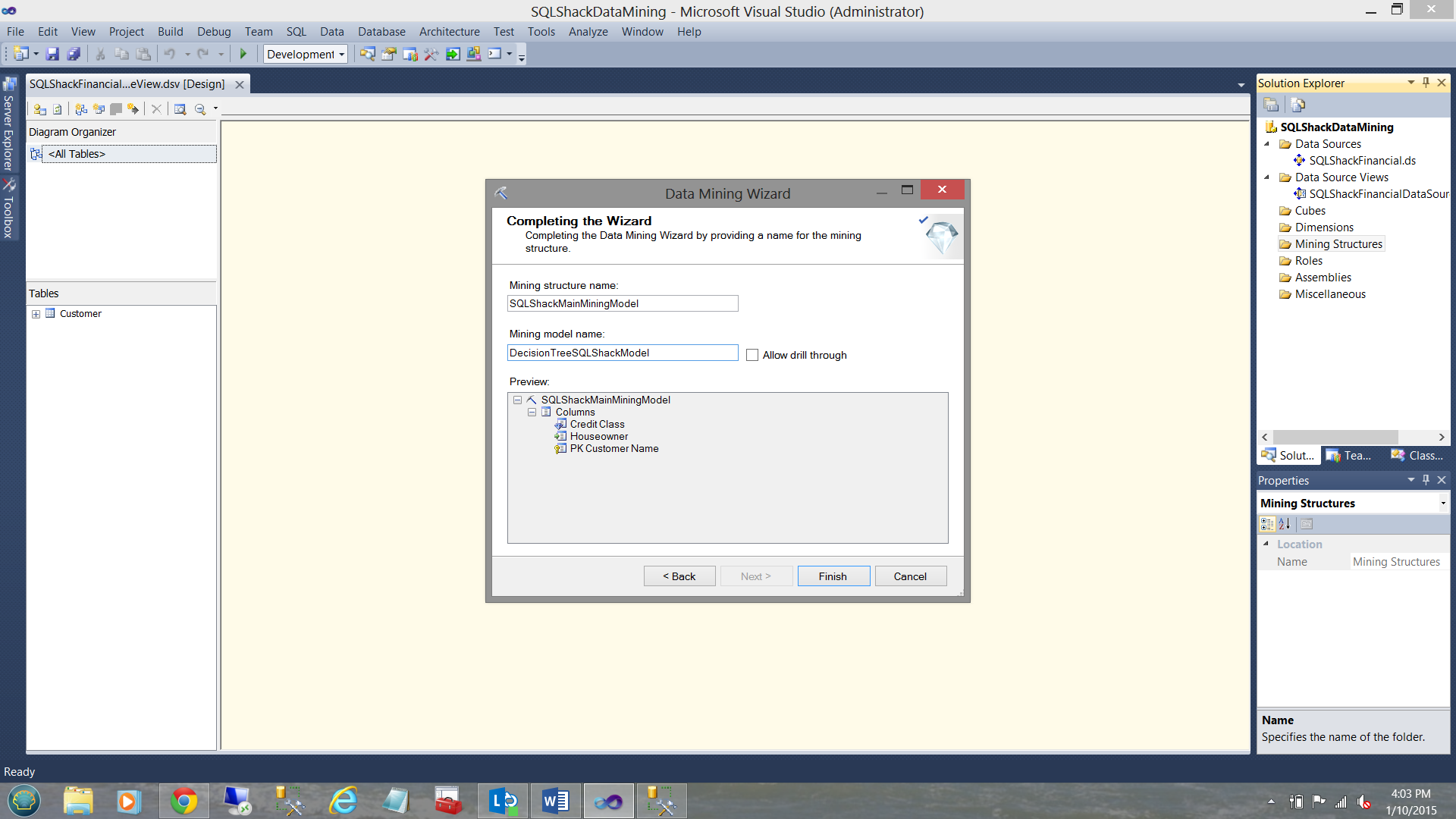
The system wants us to give our mining model a name. In this case, we choose. “SQLShackMainMiningModel”. This is the “mommy”. “SQLShackMainMiningModel” has four children, one being the Decision Tree algorithm that we just created and three more which we shall create in a few moments. For the mining model name, we select “DecisionTreeSQLShackModel”.

系统希望我们给我们的挖掘模型起一个名字。在这种情况下，我们选择。 “ SQLShackMainMiningModel”。这是“妈妈”。 “ SQLShackMainMiningModel”有四个子代，一个是我们刚创建的决策树算法，另外三个是我们稍后将创建的子代。对于挖掘模型名称，我们选择“ DecisionTreeSQLShackModel”。

We now click “Finish”.

现在，我们单击“完成”。

We are returned to our main working surface as may be seen above.

如上所示，我们回到了主要工作表面。

创建其余三个模型 ( Creating the remaining three models )

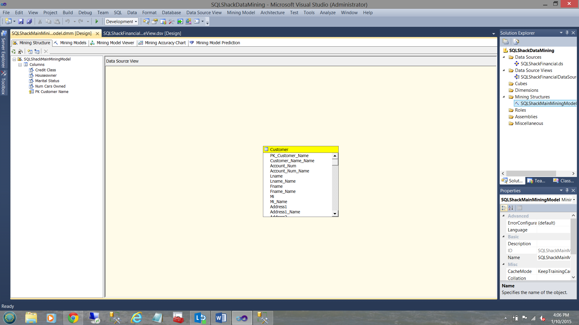
From the “Mining Structures” folder we double-click our “SQLShackMainMiningModel” that we just created.

从“挖掘结构”文件夹中，双击我们刚刚创建的“ SQLShackMainMiningModel”。

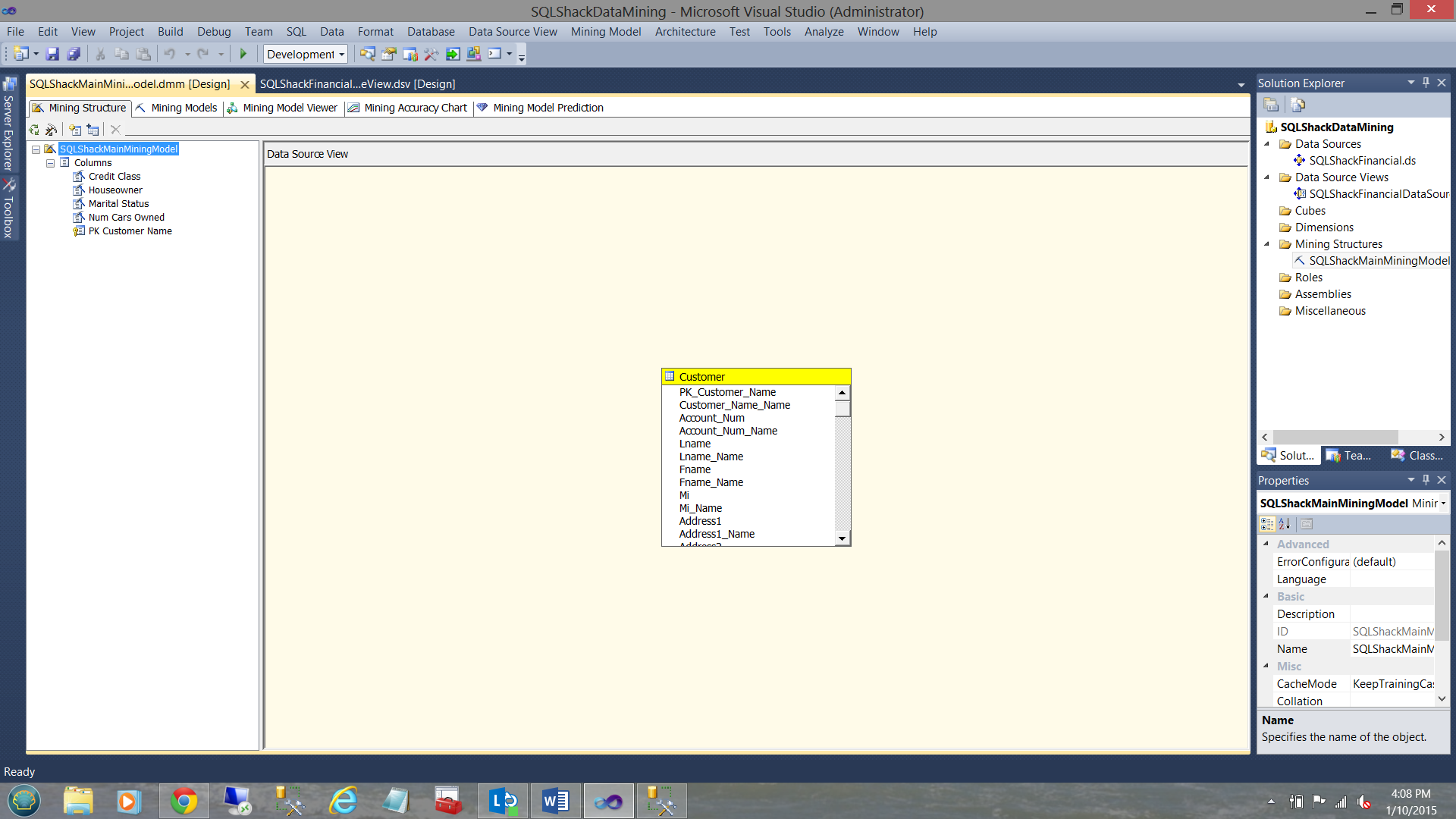
The “Mining Structure” opens. In the upper left-hand side, we can see the fields for which we opted. They are shown under the Mining structure directory (see above).

“采矿结构”打开。在左上角，我们可以看到我们选择的字段。它们显示在“采矿结构”目录下（请参见上文）。

Clicking on the “Mining Models” tab, we can see the first model that we just created.

单击“挖掘模型”选项卡，我们可以看到刚创建的第一个模型。

What we now wish to do is to create the remaining three models that we discussed above.

现在，我们要做的是创建上面讨论的其余三个模型。

The first of the three will be a Naïve-Bayes Model. This is commonly used in a predictive analysis. The principles behind the Naïve-Bayes model are beyond the scope of this paper and the reader is redirected to any good predictive analysis book.

这三个中的第一个将是朴素贝叶斯模型。这通常用于预测分析中。朴素贝叶斯模型背后的原理超出了本文的范围，读者可以重新定向到任何好的预测分析书。

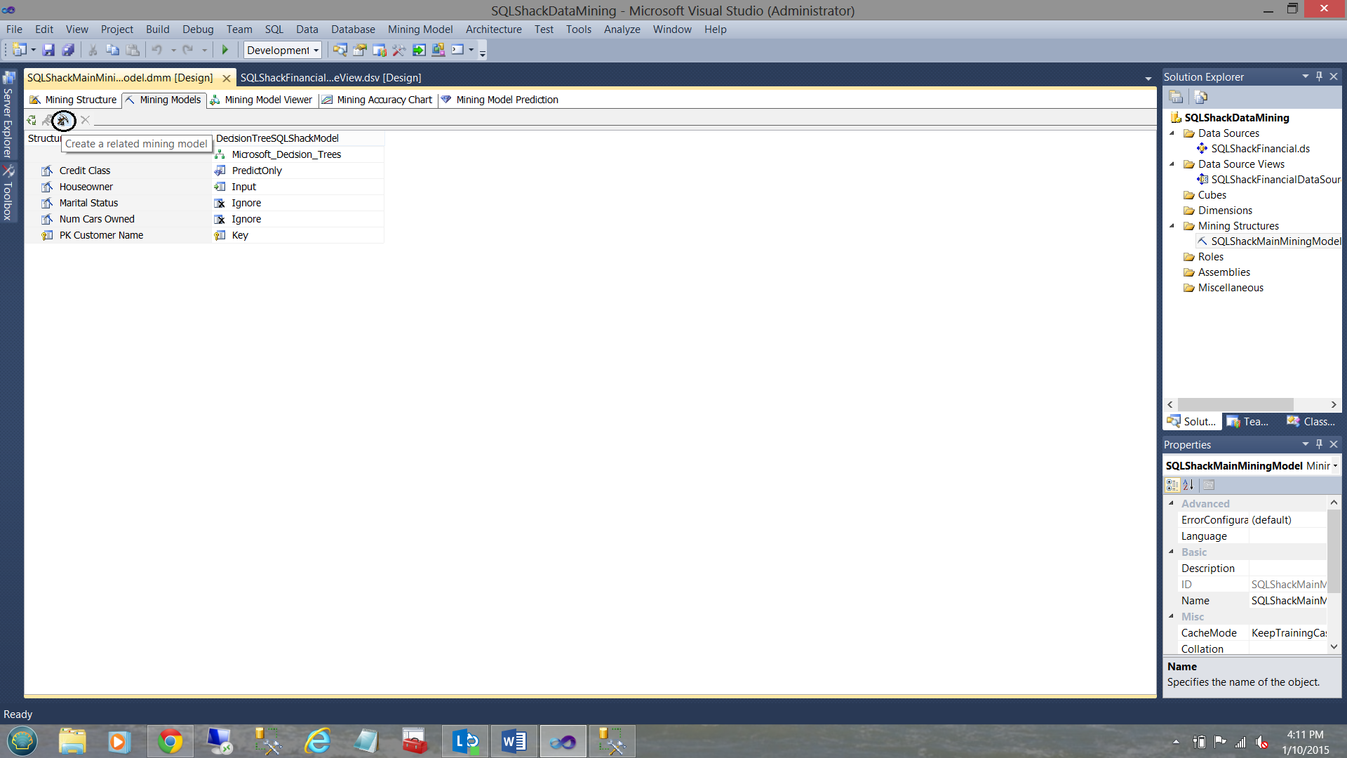
We select the “Create a related mining model” option (see above with the pick and shovel).

我们选择“创建相关的挖掘模型”选项（请参见上文中的“镐和铲”）。

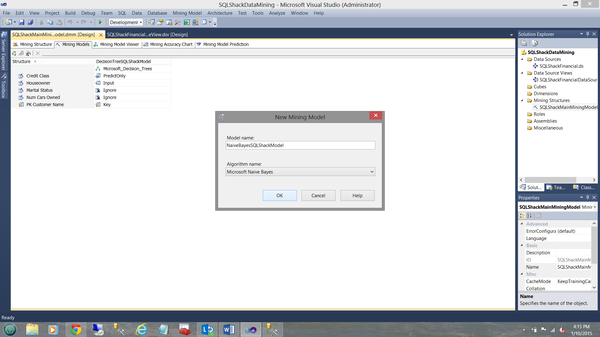
The “New Mining Model” dialogue box is brought up to be completed (see above).

弹出“ New Mining Model”对话框，以完成该操作（请参见上文）。

We give our model a name and select the algorithm type (see above).

我们给我们的模型起一个名字，然后选择算法类型（见上文）。

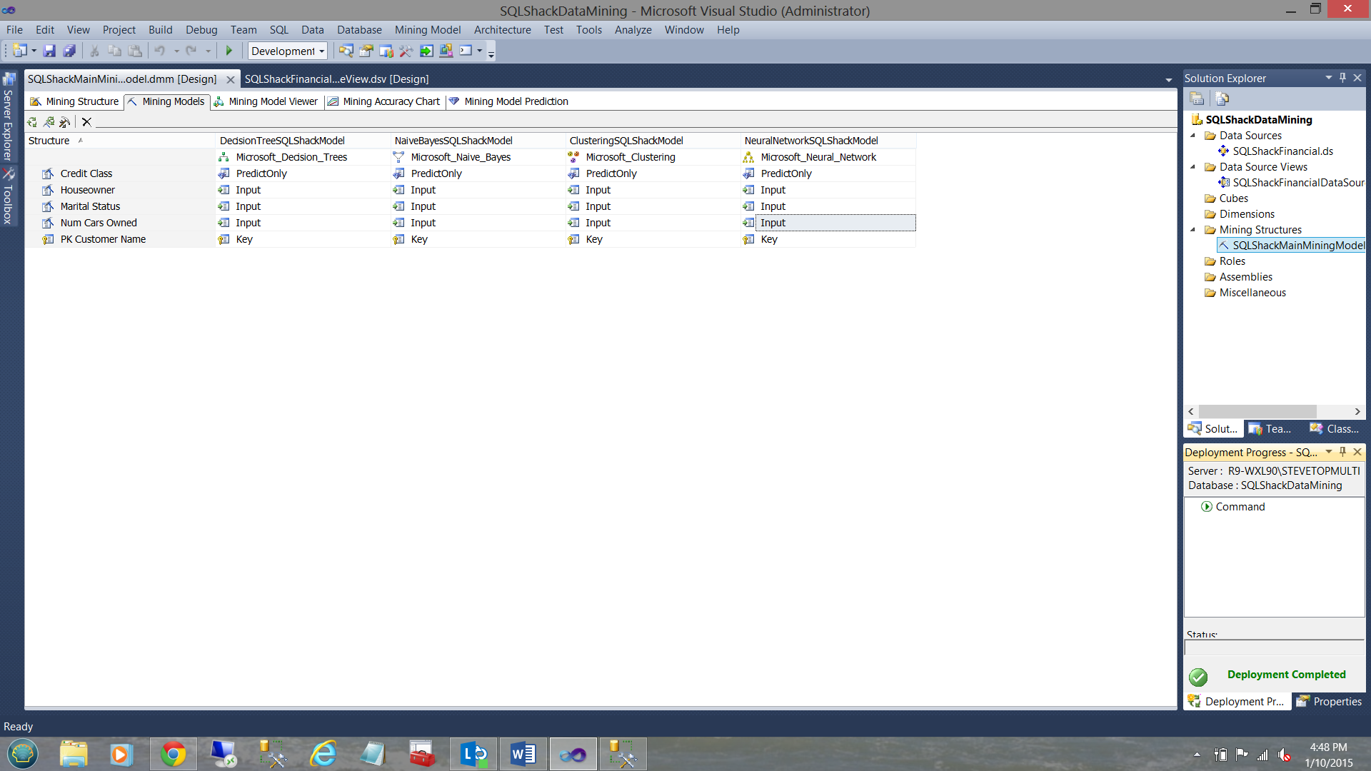
In a similar manner, we shall create a “Clustering Model” and a “Neural Network”. The final results may be seen below:

以类似的方式，我们将创建一个“聚类模型”和一个“神经网络”。最终结果如下所示：

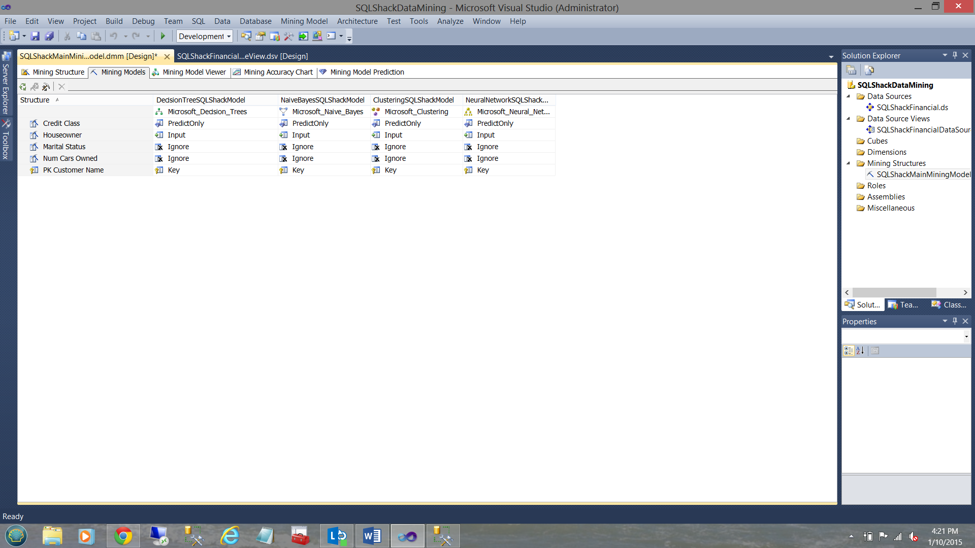
We have now completed all the heavy work and are in a position to process our models.

现在，我们已经完成了所有繁重的工作，并且能够处理我们的模型。

设置Analysis Services数据库的属性 ( Setting the properties of the Analysis Services database )

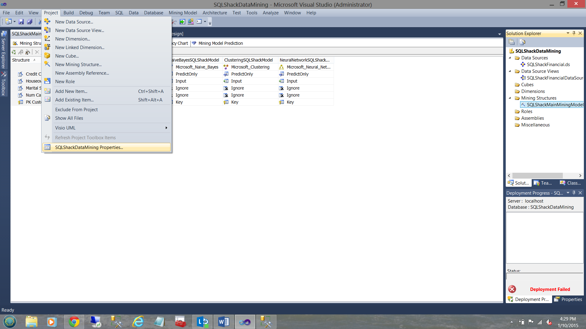
We click on the “Project” tab on the main ribbon and select “SQLShackDataMining” properties (see above).

我们单击主功能区上的“项目”选项卡，然后选择“ SQLShackDataMining”属性（请参见上文）。

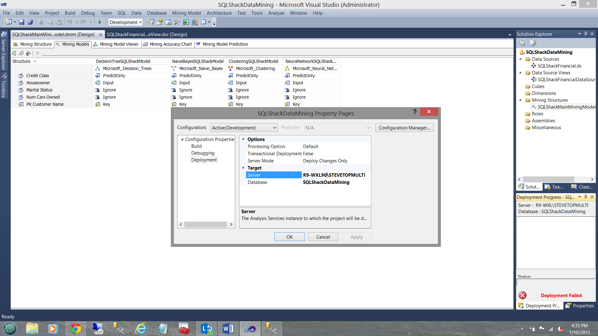
The “SQLShackDataMining Property Pages” are brought into view. Clicking on the “Deployment” tab, we select the server to which we wish to deploy our OLAP database, and in addition, give the database a name.

进入“ SQLShackDataMining属性页”。单击“部署”选项卡，我们选择希望将OLAP数据库部署到的服务器，此外，为数据库命名。

We then click “OK”.

然后，我们单击“确定”。

处理我们的模型 ( Processing our models )

We right click on the “SQLShackMainMiningModel” and select “Process”.

我们右键单击“ SQLShackMainMiningModel”，然后选择“进程”。

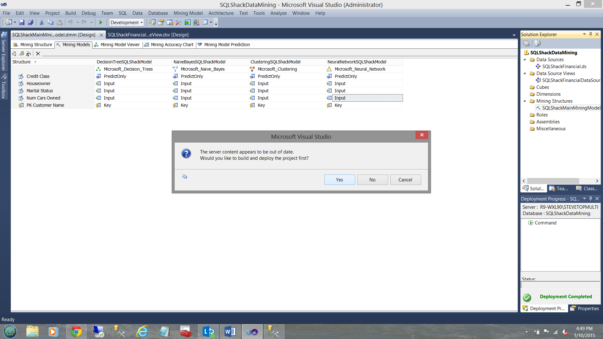
We are told that our data is old and do we want to reprocess the models (see below).

有人告诉我们我们的数据很旧，我们是否要重新处理模型（请参见下文）。

We answer “Yes”.

我们回答“是”。

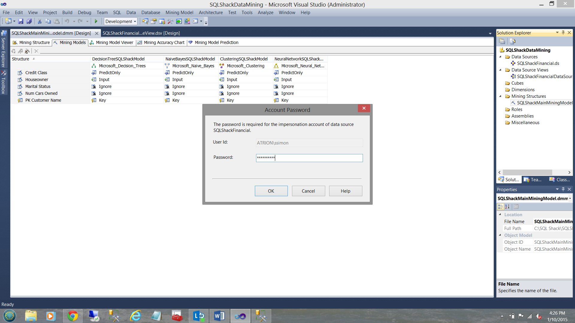
We are then asked for our credentials (see above). Once completed, we select “OK”.

然后，要求我们提供凭据（见上文）。完成后，我们选择“确定”。

One the build is complete, we are taken to the “Process Mining Structure” screen. We select the run option found at the bottom of the screen (see below in the blue oval).

一个构建完成后，我们进入“过程挖掘结构”屏幕。我们选择在屏幕底部找到的运行选项（请参见下面的蓝色椭圆形）。

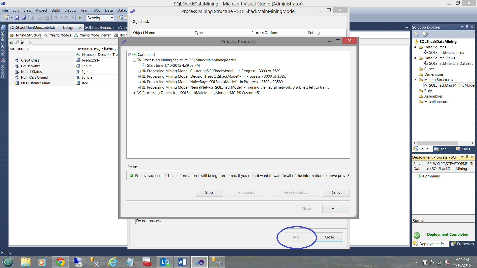
Processing occurs and the results are shown above.

进行处理，结果如上所示。

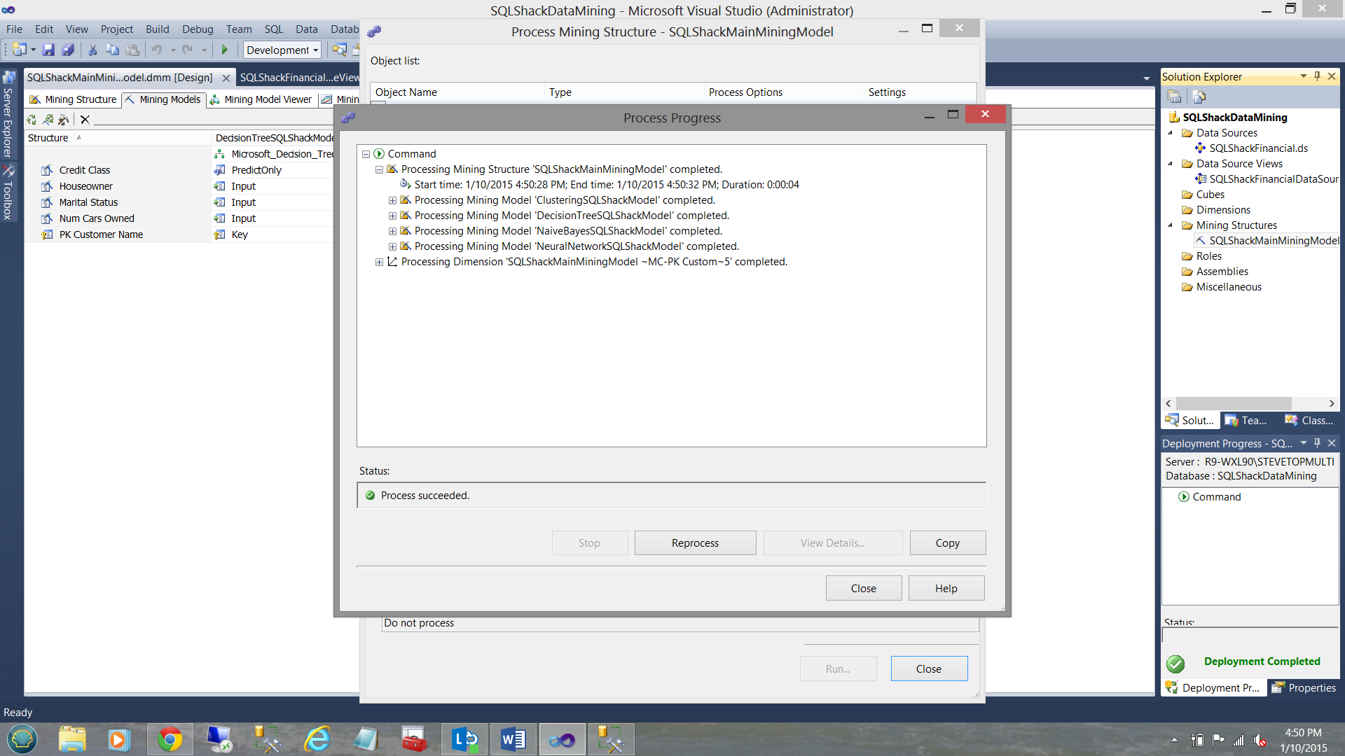
Upon completion of processing, we click the “Close” button to leave the processing routine (see above). We now find ourselves back on our work surface.

处理完成后，我们单击“关闭”按钮以退出处理例程（请参见上文）。现在，我们回到工作表面。

让乐趣开始！！ ( Let the fun begin!! )

Now that our models have been processed and tested (this occurred during the processing that we just performed), it is time to have a look at the results.

既然我们的模型已经过处理和测试（这是在我们刚刚执行的处理过程中发生的），那么现在该看看结果了。

We click on the third tab “Mining Model Viewer”

我们点击第三个标签“ Mining Model Viewer”

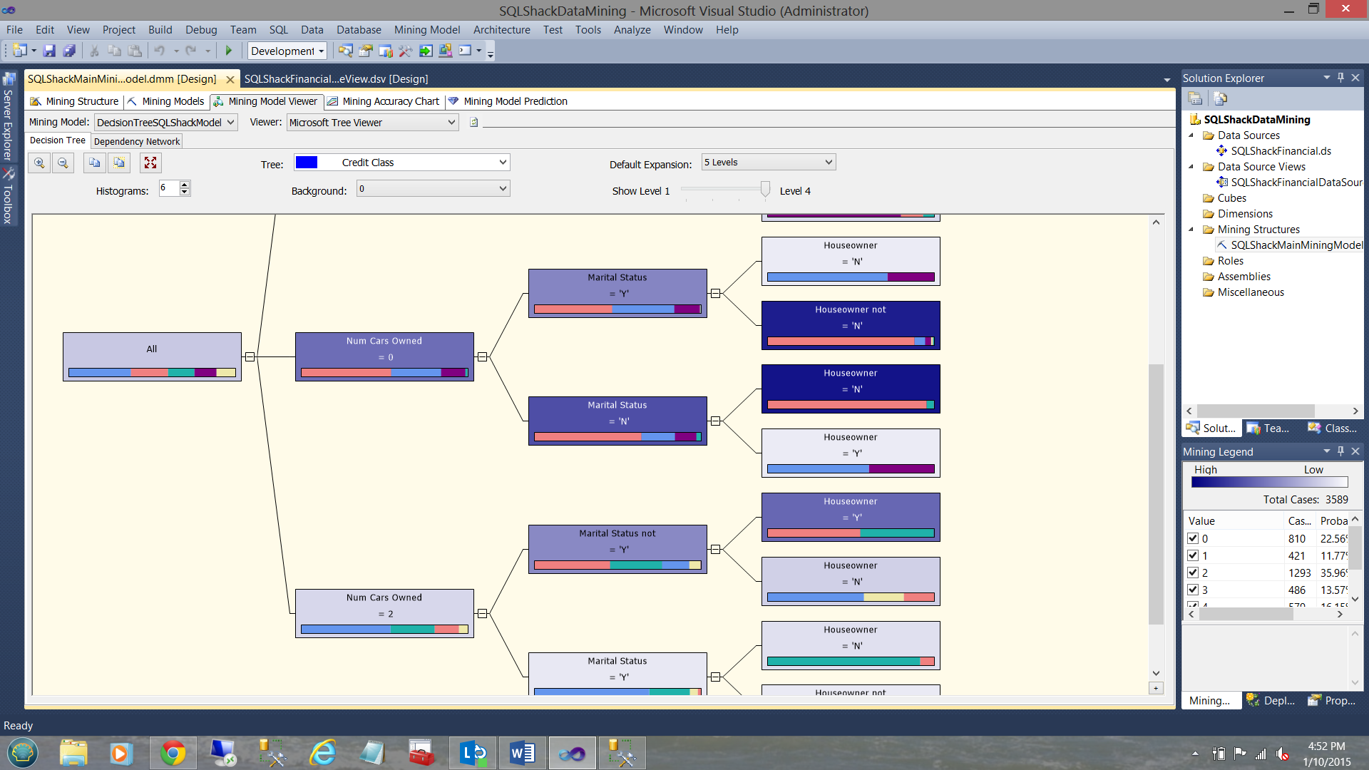
Selecting our “Decision Tree” model as a starting point, we select zero as our background value. The astute reader will remember that zero is the best risk from our lending department. THE DARKER THE COLOUR OF THE BOXES is the direction that we should be following (according to the predicted results of the processing).

选择“决策树”模型作为起点，我们选择零作为背景值。精明的读者会记住，零是我们贷款部门的最大风险。暗箱颜色是我们应该遵循的方向（根据处理的预测结果）。

That said, we should be looking at folks who own no cars, are not married and do not own a house. You say weird!! Not entirely. It can indicate that the person has no debt. We all know what happens after getting married and having children to raise