Theory for the information-based decomposition of stock price

文章目录

Motivation
The potential of Brogaard Decomposition
Intuitions for Brogaard decomposition
Technique details in Brogaard decomposition
- Define the VAR system
- Identify the VAR system
- Variance decomposition
Summary
Main References

Motivation

Brogaard et al. (2022, RFS) proposed a new variance decomposition method (hereafter I call it Brogaard decomposition) for stock price volatility, which might be a powerful tool for both accounting and market micro-structure scholars to evaluate the impacts of informatinonal shocks on stock price informativeness. In this blog, I will introduce the potential and intuition of Brogaard decomposition, as well as the theory techniques embedded in this decomposition method.

The potential of Brogaard Decomposition

The method of Brogaard Decomposition provides a novel way to distinguish the roles of different types of information (e.g., market-wide information, firm-specific private information, firm-specific public information) and noise in stock price movements. This could be relevant for both accounting scholars, who focus on the micro firm-specific movements, and market micro-structure scholars, who have apparent interests in analyzing how do different informational arrangements in the market affect the price informativeness. Beyond that, one can aggregate the model outputs both in cross section and in time series, cultivating more macro insights on how does the overall market efficiency evolve over time.

Actually, Brogaard et al. (2022, RFS) has illustrated its potential through various tests. For example, by analyzing the time trend of the noise proportion in stock return variance, they show that market efficiency is dynamic, and is heavily influenced by the environment/market structure. Specifically, they find that the proportion of noise part in stock return movement is significantly responsive to a list of material changes in market microstructure like such as the exogenous decreases in tick size. Similarly, the proportion of firm-specific information part significantly increased after the implementation of Regulation Fair Disclosure (2000) and Sarbanes-Oxley Act (2022), both having increased the quality and quantity of corporate disclosure.

Moreover, as a powerful response to the recent concern that the prevalence of high-frequency trading and passive investment may dampen the degree of which firms’ prices reflect their idiosyncratic information (e.g., Baldauf and Mollner, 2020; Lee, 2020), Brogaard et al. (2022, RFS) show that the proportion of firm-specific information accounts in stock volatility didn’t see a significant decay in the last decade, when the concerning high-frequency trading as well as passive investment became prevalent.

Last but not least, as the price variance decomposition in Brogaard et al. (2022, RFS) is actually conducted in firm level, this method could also empower both the cross-sectional and time-series comparasion among different firms, which is particularly an important feature for accounting scholars. For example, Brogaard et al. (2022, RFS) show that while there is an on average increase in price changes attributed to firm-specific shocks since 2000s, such price improvement is mainly driven by large firms.

Figure 1: Trend of Various Information Parts in Stock Volatility

Intuitions for Brogaard decomposition

Following the spirit of Beveridge and Nelson (1991), Brogaard et al. (2022, RFS) perceive that an informational shock should cause the stock price to adjust both permanently and transiently. For example, a sudden burst of unexpected buying of a stock, which is perceived as a shock to firm-specific private information by Brogaard et al. (2022, RFS), typically causes the stock price to temporarily overreact and then subsequently revert to a new equilibrium level through time. Suppose it takes 10 period for the stock price to adjust to a new equilibrium price, then the difference between the 10-step-forward price and the price just before the informational shock arrives should be the permanent price adjustment attributed to the informational shock. Correspondingly, the difference between the temporary price and the new equilibrium price is the transient noise part. Brogaard et al. (2022, RFS) showed that such intuition also applies to price underreaction, arrivals of concurrent informational shocks, as well as dynamically arrived informational shocks.

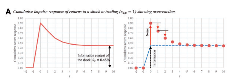
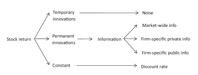
Figure 2: Intuition for Brogaard Decomposition (Overreaction)

Having established the idea to identify the impact of informational shocks on stock price adjustment, Brogaard et al. (2022, RFS) partitioned the information impounded into stock prices into three sources, and anything left over is called pricing error and is attributed to noises.

market-wide information, with the corresponding innovation term $εrm,t\varepsilon_{r_m, t}$ - private firm-specific information incorporated through trading, with the corresponding innovation term $εx,t\varepsilon_{x, t}$ - and public firm-specific information such as firm-specific news disseminated in company announcements and by the media, with the corresponding innovation term $εr,t\varepsilon_{r, t}$
By doing this, Brogaard et al. (2022, RFS) decompose the stock returns into four parts

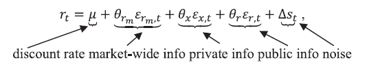
where $θrmεrm,t\theta_{r_m} \varepsilon_{r_m, t}$ captures the market-wide information incorporated into stock prices, $θxεx,t\theta_x \varepsilon_{x, t}$ captures the firm-specific private information revealed through submitted orders, and $θrεr,t\theta_r \varepsilon_{r, t}$ is the remaining part of firm-specific information that is not captured by trading on private information. $Δst\Delta s_t$ represents changes in the pricing errors.

Figure 3: Decision Tree of Brogaard Decomposition

Correspondingly, the variance of the realized stock returns $σr2\sigma_r^2$ is composed of the following four parts:
$=σs2.\begin{aligned} \text { MktInfo } &=\theta_{r_m}^2 \sigma_{\varepsilon_{r_m}}^2 \\ \text { PrivateInfo } &=\theta_x^2 \sigma_{\varepsilon_x}^2 \\ \text { PublicInfo } &=\theta_r^2 \sigma_{\varepsilon_r}^2 \\ \text { Noise } &=\sigma_s^2 . \end{aligned}\notag$ Normalizing these variance components to sum to 100% gives variance shares:
$=σs2/(σw2+σr2).\begin{aligned} \text { MktInfoShare } &=\theta_{r_m}^2 \sigma_{\varepsilon_{r_m}}^2 /(\sigma_w^2+\sigma_r^2 )\\ \text { PrivateInfoShare } &=\theta_{x}^2 \sigma_{\varepsilon_x}^2 /(\sigma_w^2+\sigma_r^2 ) \\ \text { PublicInfoShare } &=\theta_r^2 \sigma_{\varepsilon_r}^2 /(\sigma_w^2+\sigma_r^2 ) \\ \text { NoiseShare } &=\sigma_s^2 /(\sigma_w^2+\sigma_r^2 ) . \end{aligned} \notag$ where the variance of the realized stock returns $σr2\sigma_r^2$ is the combination of the variance induced by informational shocks $σw2\sigma_w^2$ and the variance attributed by noises $σs2\sigma_s^2$ .
$σr2=σw2+σs2\sigma_r^2 = \sigma_w^2+\sigma_s^2 \notag$

Technique details in Brogaard decomposition

Define the VAR system

The system in Brogaard et al. (2022, RFS) is defined by a structural VAR with 3 variables and 5 lags

$rm,t=∑l=15a1,lrm,t−l+∑l=15a2,lxt−l+∑l=15a3,lrt−l+εrm,tr_{m, t} =\sum_{l=1}^5 a_{1, l} r_{m, t-l}+\sum_{l=1}^5 a_{2, l} x_{t-l}+\sum_{l=1}^5 a_{3, l} r_{t-l}+\varepsilon_{r_m, t}$
$xt=∑l=05b1,lrm,t−l+∑l=15b2,lxt−l+∑l=15b3,lrt−l+εx,tx_t =\sum_{l=0}^5 b_{1, l} r_{m, t-l}+\sum_{l=1}^5 b_{2, l} x_{t-l}+\sum_{l=1}^5 b_{3, l} r_{t-l}+\varepsilon_{x, t}$
$rt=∑l=05c1,lrm,t−l+∑l=05c2,lxt−l+∑l=15c3,lrt−l+εr,t(B1)r_t =\sum_{l=0}^5 c_{1, l} r_{m, t-l}+\sum_{l=0}^5 c_{2, l} x_{t-l}+\sum_{l=1}^5 c_{3, l} r_{t-l}+\varepsilon_{r, t}\tag{B1}$
where

$r_{m,t}$ is the market return, the corresponding innovation $εrm,t\varepsilon_{r_{m,t}}$ represents innovations in market-wide information
$x_t$ is the signed dollar volume of trading in the given stock, the corresponding innovation $εx,t\varepsilon_{x,t}$ represents innovations in firm-specific private information
$r_t$ is the stock return, the corresponding innovation $εr,t\varepsilon_{r,t}$ represents innovations in firm-specific public information
the authors assume that $εrm,t,εx,t,εr,t\\{\varepsilon_{r_m, t}, \varepsilon_{x, t}, \varepsilon_{r, t}\\}$ are contemporaneously uncorrelated

Identify the VAR system

first estimate the reduced-form version of the VAR model

$rm,t=a0∗+∑l=15a1,l∗rm,t−l+∑l=15a2,l∗xt−l+∑l=15a3,l∗rt−l+erm,txt=b0∗+∑l=15b1,l∗rm,t−l+∑l=15b2,l∗xt−l+∑l=15b3,l∗rt−l+ex,trt=c0∗+∑l=15c1,l∗rm,t−l+∑l=15c2,l∗xt−l+∑l=15c3,l∗rt−l+er,t(B2)\begin{aligned} &r_{m, t}=a_0^*+\sum_{l=1}^5 a_{1, l}^* r_{m, t-l}+\sum_{l=1}^5 a_{2, l}^* x_{t-l}+\sum_{l=1}^5 a_{3, l}^* r_{t-l}+e_{r_m, t} \\ &x_t=b_0^*+\sum_{l=1}^5 b_{1, l}^* r_{m, t-l}+\sum_{l=1}^5 b_{2, l}^* x_{t-l}+\sum_{l=1}^5 b_{3, l}^* r_{t-l}+e_{x, t} \\ &r_t=c_0^*+\sum_{l=1}^5 c_{1, l}^* r_{m, t-l}+\sum_{l=1}^5 c_{2, l}^* x_{t-l}+\sum_{l=1}^5 c_{3, l}^* r_{t-l}+e_{r, t} \end{aligned} \tag{B2}$

impose Cholesky decomposition, forcing all elements above the principal diagonal of $B^{-1}$ to be 0 so that the system can be exactly identified

$[erm,tex,ter,t]=[100b1,010b2,0b2,11][εrm,tεx,tεr,t](B3)\left[\begin{array}{l} e_{r_m, t} \\ e_{x, t} \\ e_{r, t} \end{array}\right]=\left[\begin{array}{lll} 1 & 0 & 0 \\ b_{1,0} & 1 & 0 \\ b_{2,0} & b_{2,1} & 1 \end{array}\right]\left[\begin{array}{l} \varepsilon_{r_m, t} \\ \varepsilon_{x, t} \\ \varepsilon_{r, t} \end{array}\right]\tag{B3}$
erm,tex,ter,t
=
1b1,0b2,001b2,1001

εrm,tεx,tεr,t
(B3)
these imposed restrictions imply
- the market return $r_m$ is not contemporaneously affected by innovations in individual returns $εr,t\varepsilon_{r,t}$ or individual order imbalance/trading volume $εx,t\varepsilon_{x,t}$ - the individual order imbalance/trading volume is not contemporaneously affected by innovations in individual stock return $εr,t\varepsilon_{r,t}$
the equation (B3) implies

$erm,t=εrm,tex,t=εx,t+b1,0εrm,t=εx,t+b1,0erm,t(B4)\begin{gathered} e_{r_m, t}=\varepsilon_{r_m, t} \\ e_{x, t}=\varepsilon_{x, t}+b_{1,0} \varepsilon_{r_m, t}=\varepsilon_{x, t}+b_{1,0} e_{r_m, t} \end{gathered}\tag{B4}$
for ease of estimation, to write $e_{r,t}$ as the function of $e_{r_m,t}$ and $e_{x,t}$
$er,t=c1,0erm,t+c2,0ex,t+εr,t(B5)e_{r,t}=c_{1,0} e_{r_m, t}+c_{2,0} e_{x, t}+\varepsilon_{r, t} \tag{B5}$
plug (B4) into (B5) and get

$er,t=εr,t+(c1,0+c2,0b1,0)εrm,t+c2,0εx,t(B6)e_{r,t}=\varepsilon_{r, t}+\left(c_{1,0}+c_{2,0} b_{1,0}\right) \varepsilon_{r_m, t}+c_{2,0} \varepsilon_{x, t} \tag{B6}$
thus
- regress $e_{x,t}$ on $e_{r_m,t}$ , one can get $b_{1,0}$
- regress $e_{r,t}$ on $e_{r_m,t}$ , one can get $c_{1,0}$
- regress $e_{r,t}$ on $e_{x,t}$ , one can get $c_{2,0}$
- note that $e_{x,t}$ , $e_{r,t}$ , $e_{r,t}$ are residuls estimated from the reduced-form VAR system (B2)
with the estimated parameters $b_{1,0}, c_{1,0},c_{2,0}$ and the estimated variances of the reduced-form residuals $σer2)\left(\sigma_{e_{r_m}}^2, \sigma_{e_x}^2, \text { and } \sigma_{e_r}^2\right)$ , one can obtain the variances of the innovation terms based on equation (B4) and (B6)

$σεrm2=σerm2σεx2=σex2−b1,02σerm2σεr2=σer2−(c1,02+2c1,0c2,0b1,0)σerm2−c2,02σex2.(B7)\begin{aligned}\sigma_{\varepsilon_{r_m}}^2 &=\sigma_{e_{r_m}}^2 \\ \sigma_{\varepsilon_x}^2 &=\sigma_{e_x}^2-b_{1,0}^2 \sigma_{e_{r_m}}^2 \\ \sigma_{\varepsilon_r}^2 &=\sigma_{e_r}^2-\left(c_{1,0}^2+2 c_{1,0} c_{2,0} b_{1,0}\right) \sigma_{e_{r_m}}^2-c_{2,0}^2 \sigma_{e_x}^2 .\end{aligned} \tag{B7}$
where

$σεr2=σer2−(c1,0+c2,0b1,0)2σerm2−c2,02(σex2−b1,02σerm2)\sigma_{\varepsilon_r}^2=\sigma_{e_r}^2-\left(c_{1,0}+c_{2,0} b_{1,0}\right)^2\sigma_{e_{r_m}}^2-c_{2,0}^2(\sigma_{e_x}^2-b_{1,0}^2 \sigma_{e_{r_m}}^2)$
the impulse response can be generically conducted with the exactly identified VAR system

Variance decomposition

the cumulative return response to each of the innovations $εrm,t,εx,t,εr,t\varepsilon_{r_m, t}, \varepsilon_{x, t}, \varepsilon_{r, t}$ at $t$ =15 (point at which the authors believe the responses are generally stable) gives estimates of $θrm,θx,θr\theta_{r_m}, \theta_x, \theta_r$ respectively
in particular, the 15-step-ahead forecast error for stock return is

$rt+15−Etrt+15=ϕ31(0)εrmt+15+ϕ31(1)εrmt+15−1+⋯+ϕ31(14)εrmt+1+ϕ32(0)εxt+15+ϕ32(1)εxt+15−1+⋯+ϕ32(14)εxt+1+ϕ33(0)εrt+15+ϕ33(1)εrt+15−1+⋯+ϕ33(14)εrt+1\begin{aligned}r_{t+15}- E_t r_{t+15}&=\phi_{31}(0) \varepsilon_{r_m t+15}+\phi_{31}(1) \varepsilon_{r_m t+15-1}+\cdots+\phi_{31}(14) \varepsilon_{r_m t+1} \\ &+\phi_{32}(0) \varepsilon_{xt+15}+\phi_{32}(1) \varepsilon_{xt+15-1}+\cdots+\phi_{32}(14) \varepsilon_{xt+1} \\ &+\phi_{33}(0) \varepsilon_{rt+15}+\phi_{33}(1) \varepsilon_{rt+15-1}+\cdots+\phi_{33}(14) \varepsilon_{rt+1} \end{aligned}$
the 15-step-ahead forecast error variance of $r_{t+15}$ should contain

$θrmσεrm2+θxσεx2+θrσεr2=σεrm2[ϕ31(0)2+ϕ31(1)2+⋯+ϕ31(14)2]+σεx2[ϕ32(0)2+ϕ32(1)2+⋯+ϕ32(14)2]+σεr2[ϕ31(0)2+ϕ31(1)2+⋯+ϕ31(14)2]\begin{aligned}\theta_{r_m}\sigma_{\varepsilon_{r_m}}^2+\theta_{x}\sigma_{\varepsilon_{x}}^2+\theta_{r}\sigma_{\varepsilon_{r}}^2&=\sigma_{\varepsilon_{r_m}}^2\left[\phi_{31}(0)^2+\phi_{31}(1)^2+\cdots+\phi_{31}(14)^2\right]\\ &+\sigma_{\varepsilon_x}^2\left[\phi_{32}(0)^2+\phi_{32}(1)^2+\cdots+\phi_{32}(14)^2\right]\\ &+\sigma_{\varepsilon_r}^2\left[\phi_{31}(0)^2+\phi_{31}(1)^2+\cdots+\phi_{31}(14)^2\right]\end{aligned}$

anything left in $σr2(15)\sigma_r^2 (15)$ is attributed to noises

Summary

In this blog, I firstly discussed the potential of the variance decomposition method developed by Brogaard et al. (2022, RFS). Then I illustrate the intuition as well as the theoretical techniques employed by the Brogaard decomposition.

Main References

Baldauf, Markus, and Joshua Mollner. “High‐frequency trading and market performance.” The Journal of Finance 75.3 (2020): 1495-1526.
Bernanke, Ben S. “Alternative explanations of the money-income correlation.” (1986).
Beveridge, Stephen, and Charles R. Nelson. “A new approach to decomposition of economic time series into permanent and transitory components with particular attention to measurement of the ‘business cycle’.” Journal of Monetary Economics 7, no. 2 (1981): 151-174.
Blanchard, Olivier J., and Danny Quah. “The Dynamic Effects of Aggregate Demand and Supply Disturbances.” The American Economic Review 79, no. 4 (1989): 655-673.
Enders, Walter. “Applied Econometric Time Series. 2th ed.” New York (US): University of Alabama (2004).
Lee, Jeongmin. “Passive investing and price efficiency.” Available at SSRN 3725248 (2020).
Sims, Christopher A. “Macroeconomics and reality.” Econometrica (1980): 1-48.