Note: This is an update to my previous article Forecasting Average Daily Rate Trends for Hotels Using LSTM. I since recognised a couple of technical errors in the original analysis, and decided to write a new article to address these and expand my prior analysis.

注意：这是对我以前的文章 使用LSTM预测酒店平均每日房价趋势 的更新 。 从那以后，我认识到原始分析中的几个技术错误，因此决定写一篇新文章来解决这些问题并扩展我的先前分析。

背景 (Background)

The purpose of using an LSTM model in this instance is to forecast ADR (average daily rate) for a hotel.

在这种情况下，使用LSTM模型的目的是预测酒店的ADR(平均每日房价)。

ADR is calculated as follows:

ADR计算如下：

ADR = Revenue ÷ sold rooms

In this example, the average ADR for customers per week is calculated and formulated into a time series. The LSTM model is then used to forecast this metric on a week-by-week basis.

在此示例中，每周客户的平均ADR被计算并制定为时间序列。 然后，将LSTM模型用于每周一次预测该指标。

The original study by Antonio, Almeida and Nunes (2016) can be found here.

Antonio，Almeida和Nunes(2016)的原始研究可在此处找到。

Using pandas, the average ADR is calculated per week. Here is a plot of the weekly ADR trend.

使用大熊猫，每周平均ADR会计算出来。 这是每周ADR趋势图。

Note that the Jupyter Notebook for this example is available at the end of this article.

请注意，本文结尾处提供了此示例的Jupyter Notebook。

资料准备 (Data Preparation)

1.使用MinMaxScaler规范化数据 (1. Normalizing data with MinMaxScaler)

As with any neural network, the data needs to be scaled for proper interpretation by the network, a process known as normalization. MinMaxScaler is used for this purpose.

与任何神经网络一样，需要对数据进行缩放以由网络进行适当的解释，这一过程称为规范化。 MinMaxScaler用于此目的。

However, this comes with a caveat. Scaling must be done after the data has been split into training, validation and test sets — with each being scaled separately. A common mistake when first using the LSTM (I made this mistake myself) is to first normalize the data before splitting the data.

但是，这带有警告。 在将数据划分为训练集，验证集和测试集之后 ，必须进行缩放-分别对每个缩放。 第一次使用LSTM时(我自己犯了这个错误)，一个常见的错误是在拆分数据之前先对数据进行规范化。

The reason this is erroneous is that the normalization technique will use data from the validation and test sets as a reference point when scaling the data as a whole. This will inadvertently influence the values of the training data, essentially resulting in data leakage from the validation and test sets.

这是错误的原因是，在对数据进行整体缩放时，规范化技术将使用来自验证和测试集的数据作为参考点。 这将无意中影响训练数据的值，从而实质上导致验证和测试集的数据泄漏。

In this regard, 100 data points are split into training and validation sets, with the last 15 data points being held as test data for comparison with the LSTM predictions.

在这方面，将100个数据点分为训练和验证集，最后15个数据点作为测试数据保存，以与LSTM预测进行比较。

train_size = int(len(df) * 0.8)val_size = len(df) - train_sizetrain, val = df[0:train_size,:], df[train_size:len(df),:]

A dataset matrix is formed:

形成一个数据集矩阵：

def create_dataset(df, previous=1):    dataX, dataY = [], []    for i in range(len(df)-previous-1):        a = df[i:(i+previous), 0]        dataX.append(a)        dataY.append(df[i + previous, 0])    return np.array(dataX), np.array(dataY)

At this point, the training data can be scaled as follows:

此时，训练数据可以按如下比例缩放：

scaler = MinMaxScaler(feature_range=(0, 1))train = scaler.fit_transform(train)train

Here is a sample of the output:

这是输出示例：

array([[0.35915778],       [0.42256282],       [0.53159902],...       [0.0236608 ],       [0.11987636],       [0.48651694]])

Similarly, the validation data is scaled in the same way:

同样，验证数据的缩放方式也相同：

val = scaler.fit_transform(val)val

2.定义回溯期 (2. Define lookback period)

A “lookback period” defines how many previous timesteps are used in order to predict the subsequent timestep. In this regard, we are using a one-step prediction model.

“回溯期”定义了使用多少个先前的时间步长来预测随后的时间步长。 在这方面，我们使用了一个单步预测模型。

The lookback period is set to 5 in this instance. This means that we are using the time steps at t-4, t-3, t-2, t-1, and t to predict the value at time t+1.

在这种情况下，回溯期设置为5 。 这意味着我们将使用t-4，t-3，t-2，t-1和t处的时间步长来预测时间t + 1处的值。

# Lookback periodlookback = 5X_train, Y_train = create_dataset(train, lookback)X_val, Y_val = create_dataset(val, lookback)

Note that the selection of the lookback period is quite an arbitrary process. In this instance, a lookback window of 5 was shown to demonstrate the best predictive performance on the test set. However, another option could be to use the number of lags as indicated by PACF to set the size of the lookback window, as described at Data Science Stack Exchange.

注意，回溯期的选择是一个相当随意的过程。 在这种情况下，回溯窗口显示为5，以证明测试集具有最佳的预测性能。 但是，另一个选择可能是使用PACF指示的延迟数来设置回溯窗口的大小，如Data Science Stack Exchange中所述 。

Let’s take a look at the normalized window for X_train.

让我们看一下X_train的标准化窗口。

array([[0.35915778, 0.42256282, 0.53159902, 0.6084246 , 0.63902841],       [0.42256282, 0.53159902, 0.6084246 , 0.63902841, 0.70858066],       [0.53159902, 0.6084246 , 0.63902841, 0.70858066, 0.75574219],...

Here are the first three entries. We can see that the five time steps immediately prior to the one we are trying to predict move in a stepwise motion.

这是前三个条目。 我们可以看到紧接我们试图预测逐步运动的五个时间步长。

For instance, the first entry shows 0.63902841 at time t. In the second entry, this value now moves backwards to time t-1.

例如，第一项在时间t显示0.63902841。 在第二个条目中，此值现在向后移到时间t-1 。

Let’s give an example applicable to this situation. For a hotel that wishes to predict the ADR value in week 26 for instance, the hotel will use this model to make the prediction in the prior week using data for weeks 21, 22, 23, 24, and 25.

让我们举一个适用于这种情况的例子。 例如，对于希望在第26周预测ADR值的酒店，该酒店将使用该模型使用第21、22、23、24和25周的数据在前一周进行预测。

Now, the input is reshaped into a [samples, time steps, features] format.

现在，输入被重塑为[样本，时间步长，特征]格式。

# reshape input to be [samples, time steps, features]X_train = np.reshape(X_train, (X_train.shape[0], 1, X_train.shape[1]))X_val = np.reshape(X_val, (X_val.shape[0], 1, X_val.shape[1]))

In this case, the shape of the input is [74, 1, 1].

在这种情况下，输入的形状为[74，1，1] 。

74 samples are present in the training data, the model is operating on a time step of 1, and 1 feature is being used in the model, i.e. a lagged version of the time series.

训练数据中存在74个样本，该模型以1的时间步长运行，并且模型中使用了1个特征，即时间序列的滞后版本。

LSTM建模 (LSTM Modelling)

An LSTM model is defined as follows:

LSTM模型定义如下：

# Generate LSTM networkmodel = tf.keras.Sequential()model.add(LSTM(4, input_shape=(1, lookback)))model.add(Dense(1))model.compile(loss='mean_squared_error', optimizer='adam')history=model.fit(X_train, Y_train, validation_split=0.2, epochs=100, batch_size=1, verbose=2)

An LSTM model is created with 4 neurons. The mean squared error is being used as the loss function — given that we are dealing with a regression problem. Additionally, the adam optimizer is used, with training done over 100 epochs with a validation split of 20%.

用4个神经元创建一个LSTM模型。 考虑到我们正在处理回归问题，均方误差被用作损失函数。 此外，使用了adam优化程序，训练了100多个纪元，验证间隔为20％。

Here is a visual overview of the training and validation loss:

这是培训和验证损失的直观概述：

# list all data in historyprint(history.history.keys())# summarize history for accuracyplt.plot(history.history['loss'])plt.plot(history.history['val_loss'])plt.title('model loss')plt.ylabel('loss')plt.xlabel('epoch')plt.legend(['train', 'val'], loc='upper left')plt.show()

We can see that after an initial increase in the validation loss, the loss starts to decrease after about 10 epochs.

我们可以看到，在最初增加验证损失后，损失大约在10个纪元后开始减少。

Now, the predictions are converted back to the original scale:

现在，将预测转换回原始比例：

# Convert predictions back to normal valuestrainpred = scaler.inverse_transform(trainpred)Y_train = scaler.inverse_transform([Y_train])valpred = scaler.inverse_transform(valpred)Y_val = scaler.inverse_transform([Y_val])predictions = valpred

The root mean squared error is calculated on the training and validation set:

均方根误差是根据训练和验证集计算得出的：

# calculate RMSEtrainScore = math.sqrt(mean_squared_error(Y_train[0], trainpred[:,0]))print('Train Score: %.2f RMSE' % (trainScore))valScore = math.sqrt(mean_squared_error(Y_val[0], valpred[:,0]))print('Validation Score: %.2f RMSE' % (valScore))

The obtained RMSE values are as follows:

获得的RMSE值如下：

• Train error: 3.88 RMSE

  火车错误： 3.88 RMSE

• Validation error: 8.78 RMSE

  验证错误： 8.78 RMSE

With a mean ADR value of 69.99 across the validation set, the validation error is quite small in comparison (roughly 12% of the mean value), indicating that the model has done a good job at forecasting ADR values.

整个验证集的平均ADR值为69.99，相比而言，验证误差很小(约为平均值的12％)，这表明该模型在预测ADR值方面做得很好。

Here is a plot of the forecasted versus actual ADR values across the training and validation set.

这是整个训练和验证集的预测ADR值与实际ADR值的关系图。

# Plot all predictionsinversetransform, =plt.plot(scaler.inverse_transform(df))trainpred, =plt.plot(scaler.inverse_transform(trainpredPlot))valpred, =plt.plot(scaler.inverse_transform(valpredPlot))plt.xlabel('Number of weeks')plt.ylabel('Cancellations')plt.title("Predicted vs. Actual Weekly ADR")plt.show()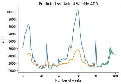

We can see that the LSTM model is generally capturing the directional oscillations of the time series. However, during periods of extreme spikes in ADR, e.g. week 60, the model seems to perform less well.

我们可以看到LSTM模型通常捕获了时间序列的方向性振荡。 但是，在ADR急剧上升的时期内(例如第60周)，该模型的效果似乎不太好。

However, in order to fully determine whether the model has predictive power — it will now be used to predict the last 15 time steps in the series, i.e. the test data.

但是，为了完全确定模型是否具有预测能力，现在将其用于预测序列中的最后15个时间步长，即测试数据。

Xnew = np.array([tseries.iloc[95:100],tseries.iloc[96:101],tseries.iloc[97:102],tseries.iloc[98:103],tseries.iloc[99:104],tseries.iloc[100:105],tseries.iloc[101:106],tseries.iloc[102:107],tseries.iloc[103:108],tseries.iloc[104:109],tseries.iloc[105:110],tseries.iloc[106:111],tseries.iloc[107:112],tseries.iloc[108:113],tseries.iloc[109:114]])

In this example, Xnew uses the previous five time steps to predict at time t+1. For instance, weeks 95 to 100 are used to predict the ADR value for week 101, then weeks 96 to 101 are used to predict week 102, and so on.

在此示例中，Xnew使用前五个时间步长预测时间t + 1 。 例如，第95到100周用于预测第101周的ADR值，然后第96到101周用于预测第102周，依此类推。

The above graph illustrates the LSTM predictions versus the actual ADR values in the test set — the last 15 points in the series.

上图显示了LSTM预测与测试集中实际ADR值的对比-系列中的最后15个点。

The obtained RMSE and MAE (mean absolute error) values are as follows:

获得的RMSE和MAE(平均绝对误差)值如下：

• MAE: -27.65

  湄： -27.65

• RMSE: 31.91

  RMSE： 31.91

The RMSE error for the test set is significantly higher than that for the validation set — which would be expected since we are working with unseen data.

测试集的RMSE错误明显高于验证集的误差-由于我们正在使用看不见的数据，因此这是可以预期的。

However, with a mean ADR value of 160 across the test set, the RMSE error is approximately 20% of the size of the mean value, indicating that the LSTM does still have reasonably strong predictive power in determining the value of the next timestep.

但是，如果整个测试集的平均ADR值为160 ，则RMSE误差约为平均值大小的20％，这表明LSTM在确定下一时间步长的值时仍具有相当强的预测能力。

Ideally, one would like to use a significantly larger data sample to validate whether the LSTM would retain predictive power across new data. Additionally, as illustrated in this Reddit thread, LSTMs can be prone to overfitting depending on the size of the data sample.

理想情况下，我们希望使用大得多的数据样本来验证LSTM是否将保留对新数据的预测能力。 此外，如此Reddit线程中所示 ，根据数据样本的大小，LSTM可能易于过度拟合。

In this regard, a larger data sample is needed to validate if this model would work in a real-world scenario. However, the preliminary results in this case look promising.

在这方面，需要更大的数据样本来验证此模型是否可以在实际场景中使用。 但是，这种情况下的初步结果看起来很有希望。

结论 (Conclusion)

In this example, you have seen:

在此示例中，您已经看到：

• How to properly format data to work with an LSTM model如何正确格式化数据以使用LSTM模型
• Building of a one-step LSTM predictive model建立一步式LSTM预测模型
• Interpretation of RMSE and MAE values to determine model accuracy解释RMSE和MAE值以确定模型准确性

Many thanks for reading, and any feedback or questions are greatly appreciated. You can find the Jupyter Notebook for this example here.

非常感谢您的阅读，非常感谢您提供任何反馈或问题。 你可以找到Jupyter笔记本这个例子在这里 。

Additionally, I also highly recommend this tutorial by Machine Learning Mastery, which was used as a guideline for designing the LSTM model used in this example.

另外，我也强烈推荐Machine Learning Mastery撰写的本教程，该教程被用作设计本示例中使用的LSTM模型的指南。

Disclaimer: This article is written on an “as is” basis and without warranty. It was written with the intention of providing an overview of data science concepts, and should not be interpreted as professional advice in any way.

免责声明：本文按“原样”撰写，不作任何担保。 它旨在提供数据科学概念的概述，并且不应以任何方式解释为专业建议。