总览 (Overview)

This post will provide a technical guide on machine learning theory within data science interviews. It is by no means comprehensive but aims to highlight key technical points within each topic. The problems discussed are from this data science interview newsletter which features questions from top tech companies and will be involved in an upcoming book.

这篇文章将在数据科学访谈中提供有关机器学习理论的技术指南。 它绝不是全面的，而是旨在强调每个主题中的关键技术点。 讨论的问题来自此数据科学访谈通讯 ，其中包含来自顶级高科技公司的问题，并将参与下一本书 。

数学先决条件 (Mathematical Prerequisites)

随机变量 (Random Variables)

Random variables are a core topic within probability and statistics, and interviewers are generally looking for an understanding of the principles and basic ability to manipulate them.

随机变量是概率和统计数据的核心主题，访调员通常希望了解其原理和基本能力。

For any given random variable X, it has the following properties (below we assume X is continuous, but the analogous holds for discrete random variables). The expectation (average value) is given by:

对于任何给定的随机变量X，它都具有以下属性(下面我们假设X是连续的，但是类似的情况适用于离散随机变量)。 期望(平均值)由下式给出：

and the variance is given by:

方差由下式给出：

For any given random variables X and Y, the covariance, a linear measure of relationship, is defined by:

对于任何给定的随机变量X和Y，协方差是关系的线性度量，定义为：

and normalization of covariance is the correlation between X and Y:

协方差的归一化是X和Y之间的相关性：

概率分布 (Probability Distributions)

There are many probability distributions, and interviewers generally aren’t testing whether you’ve memorized specific properties on each (although it is helpful to know basics), but more so that you can apply them to specific situations properly. Because of this, the most commonly discussed one in Data Science Interviews is the Normal distribution, which has many real-life applications. For a single variable the probability density is given by the following, for a mean and variance parameter:

概率分布很多，访调员通常不会测试您是否记住了每个属性(尽管有助于了解基本知识)，但是更多的是，以便您可以将它们正确地应用于特定情况。 因此，在数据科学访谈中最常讨论的是正态分布，它具有许多实际应用。 对于单个变量，均值和方差参数的概率密度如下所示：

For fitting parameters, there are two general methods. In maximum likelihood estimation (MLE) the goal is estimate the most likely parameters given a likelihood function:

对于拟合参数，有两种通用方法。 在最大似然估计(MLE)中，目标是在给定似然函数的情况下估计最可能的参数：

Since the values of X are assumed to be i.i.d, then the likelihood function becomes:

由于假设X的值是iid，则似然函数变为：

It is convenient to take logs (since log is a monotonically increasing function, maximizing the log-likelihood is equivalent to maximizing the likelihood):

取日志很方便(因为日志是单调递增的函数，所以最大化对数似然性等于最大化似然性)：

Another way of fitting parameters is through maximum a posteriori estimation (MAP), which assumes a prior distribution.

拟合参数的另一种方法是通过最大后验估计(MAP)，它采用先验分布。

where the similar log-likelihood from before applies.

适用与之前相似的对数可能性。

线性代数 (Linear Algebra)

Generally, interviewers won’t expect you to delve deeply into linear algebra unless there are specific machine learning emphases. However, it is still helpful to review basics since it helps with the understanding of various algorithms and theoretical underpinnings. There are many sub-topics within linear algebra, but one sub-topic worth discussing briefly is eigenvalues and eigenvectors. Mechanically, for some square matrix A, we have a vector x is an eigenvector of A if:

通常，除非有特定的机器学习重点，否则访问员不会期望您深入研究线性代数。 但是，复习基础知识仍然有帮助，因为它有助于理解各种算法和理论基础。 线性代数中有许多子主题，但是一个值得简要讨论的子主题是特征值和特征向量。 从机械上讲，对于某些方阵A，如果满足以下条件，则有一个向量x是A的特征向量：

Since a matrix is a linear transformation, eigenvectors are cases whereby the resulting transformation of the matrix on that vector results in the same direction as before, although with some scaling factor (the eigenvalues). There are many real-life use cases of eigenvalues and eigenvectors: for example, identifying the orientation of large datasets (discussed in PCA), or for dynamical systems (how a system oscillates and how quickly it will stabilize).

由于矩阵是线性变换，因此特征向量是矩阵在该向量上的最终变换结果与以前相同的方向的情况，尽管具有一定的比例因子(特征值)。 特征值和特征向量在现实生活中有许多用例：例如，识别大型数据集的方向(在PCA中讨论)，或用于动态系统(系统如何振荡以及如何稳定)。

The decomposition of a square matrix into its eigenvectors is called an eigendecomposition. Note that while not all matrices are square, through Singular Value Decomposition (SVD), every matrix has a decomposition:

将方阵分解为特征向量的过程称为特征分解。 请注意，尽管并非所有矩阵都是正方形，但通过奇异值分解(SVD)，每个矩阵都有一个分解：

Although the mathematical details are beyond the scope of this discussion, both eigendecomposition and SVD are worth looking into in detail before your technical interview.

尽管数学上的细节不在本文讨论的范围内，但是本征分解和SVD都值得在进行技术面试之前进行详细研究。

偏差-偏差权衡 (Bias-Variance Tradeoff)

This is a topic occasionally asked in interviews due to relevance with overfitting and model selection. With any model, we generally are trying to estimate a true underlying:

由于与过度拟合和模型选择的相关性，这是访谈中偶尔会问到的话题。 对于任何模型，我们通常都在尝试估算真实的基础：

through data where w is usually noise that is zero-mean and a Gaussian random variable. As mentioned prior, MLE and MAP are reasonable ways to deduce parameters. To assess how well the model fits, we can decompose the error of y as the following:

通过数据，其中w通常是零均值噪声和高斯随机变量。 如前所述，MLE和MAP是推断参数的合理方法。 为了评估模型的拟合程度，我们可以将y的误差分解如下：

1. bias (how well the values come close to the true underlying f(x) values)偏见(这些值接近真实的基础f(x)值的程度)
2. variance (how much the prediction changes based on training inputs)方差(根据训练输入预测值发生了多少变化)
3. irreducible error (due to inherently noisy observation processes不可减少的误差(由于固有的嘈杂的观测过程

There is a trade-off between bias and variance, and this is a useful framework for thinking about how different models operate. The overall goal is to control overfitting (and not generalizing well out of sample) to produce stable and accurate models.

偏差和方差之间需要权衡，这是思考不同模型如何运作的有用框架。 总体目标是控制过度拟合(而不是过度推广样本)以生成稳定且准确的模型。

线性回归 (Linear Regression)

This method is one of the most frequently taught methods and has many real-life applications, ranging from predicting housing prices to studying the efficacy of medical trials. Interviewers asking this are generally trying to assess your understanding of the basic formulations and occasionally the relevance of knowing some of the theory to real life applications.

这种方法是最常教授的方法之一，并且在许多实际应用中都可以使用，从预测住房价格到研究医学试验的有效性。 询问此事的面试官通常试图评估您对基本公式的理解，有时甚至是了解一些理论与现实应用之间的相关性。

In linear regression, the goal is to estimate y = f(x) of the following form:

在线性回归中，目标是估计以下形式的y = f(x)：

where X is a matrix of data points and β the vector of weights. In the least-squares context, linear regression minimizes the residual sum-of-squares (RSS), which is given by:

其中X是数据点的矩阵，β是权重的向量。 在最小二乘上下文中，线性回归将残差平方和(RSS)最小化，其公式为：

In regression, one can use MLE to estimate the β values by using a multivariate Gaussian:

在回归中，可以使用MLE通过使用多元高斯估计β值：

which leads to results that are the same as minimizing the RSS. For a MAP context, there can be priors for β, of which leads to Ridge Regression, which penalizes the weights to prevent overfitting. In Ridge regression, the objective function becomes minimizing:

这导致的结果与最小化RSS相同。 对于MAP上下文，可能有β的先验值，这会导致Ridge回归，这会惩罚权重以防止过度拟合。 在Ridge回归中，目标函数变得最小：

降维 (Dimensionality Reduction)

主成分分析 (Principal Components Analysis)

This topic is less common in interviews but is often alluded to during discussions about data-preprocessing or feature engineering. Decomposing data into a smaller set of variables is very useful for summarizing and visualizing data. This overall process is called dimensionality reduction. One common method of dimensionality reduction is Principal Components Analysis (PCA), which reconstructs data into a lower dimensional setting. It looks for a small number of linear combinations of a vector x (say it is p-dimensional) to explain the variance within x. More specifically, we want to find the vector w of weights such that we can define the following linear combination:

该主题在访谈中不太常见，但在讨论数据预处理或功能工程时经常被提及。 将数据分解为较小的变量集对于汇总和可视化数据非常有用。 这个整体过程称为降维。 降维的一种常见方法是主成分分析(PCA)，它将数据重构为较低维的设置。 它寻找向量x的少量线性组合(假设它是p维的)来解释x内的方差。 更具体地说，我们想要找到权重的向量w，以便我们可以定义以下线性组合：

subject to the following:

遵守以下规定：

Hence we have the following procedural description where first we find the first component with maximal variance, and then the second that is uncorrelated with the first, and continue this procedure iteratively. The idea is to end with say, k dimension such that

因此，我们具有以下过程描述，其中首先找到具有最大方差的第一个分量，然后找到与第一个不相关的第二个分量，然后迭代地继续此过程。 这个想法以k维结尾，这样

Using some algebra, the final result is an eigendecomposition of the covariance matrix of X, whereby the first principal component is the eigenvector corresponding to the largest eigenvalue and so on.

使用某些代数，最终结果是X的协方差矩阵的本征分解，其中第一个主成分是对应于最大本征值的本征向量，依此类推。

分类 (Classification)

通用框架 (General Framework)

Classification is commonly asked during interviews since due to the the abundance of real-life applications. Tech companies love to ask about classifying customers and users into different segments.

由于现实生活中的应用程序很多，因此在面试过程中通常会要求分类。 科技公司喜欢问有关将客户和用户划分为不同细分市场的问题。

The goal of classification is to assign a given data point to one of K classes, instead of a continuous value (as in regression), and there are two types of models. The first is generative which models the joint probability distribution between X and Y. That is, for an input X, we want to classify an arbitrary data point x with the following class label:

分类的目的是将给定的数据点分配给K个类别之一，而不是连续值(如在回归中那样)，并且有两种类型的模型。 第一个是生成式的，它对X和Y之间的联合概率分布进行建模。也就是说，对于输入X，我们希望使用以下类别标签对任意数据点x进行分类：

This joint distribution between X and Y is given by:

X和Y之间的这种联合分布由下式给出：

and for each given class k we have:

对于每个给定的类k，我们有：

The result of maximizing the posterior means there will be decision boundaries between classes where the resulting posterior probability is equal.

最大化后验的结果意味着在类之间存在决策边界，其中后验概率相等。

The second is discriminative, which directly learn a decision boundary by choosing a class that maximizes the posterior probability distribution:

第二种是判别式，它通过选择最大化后验概率分布的类来直接学习决策边界：

So both methods end up choosing a predicted class that maximize the posterior; the difference is just in the approach.

因此，这两种方法最终都选择了使后验最大化的预测类。 区别仅在于方法。

逻辑回归 (Logistic Regression)

One of the popular classification algorithms is logistic regression, and is often asked in conjunction with linear regression during interviews as a way to assess basic knowledge on classification algorithms. In logistic regression, we take a linear output and convert it to a probability between 0 and 1 using the sigmoid function:

流行的分类算法之一是逻辑回归，通常在面试时与线性回归结合使用，以评估分类算法的基础知识。 在逻辑回归中，我们采用线性输出，并使用Sigmoid函数将其转换为介于0和1之间的概率：

In matrix form, the decision looks like the following, where a 1 is the target class if the output is at least 0.5:

以矩阵形式，决策如下所示，如果输出至少为0.5，则目标类为1：

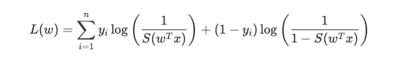
The loss function for logistic regression is the log-loss:

Logistic回归的损失函数为对数损失：

Note that the posterior is being modeled directly and hence logistic regression is a discriminative model.

请注意，后验直接建模，因此逻辑回归是一种判别模型。

线性判别分析 (Linear Discriminant Analysis)

Linear Discriminant Analysis (LDA) is not a commonly asked topic during interviews but serves as an interesting topic to know since it is a generative model rather than a discriminative model (which logistic regression was). It assumes that given some class k, the distribution of any data from that class follows a multivariate Gaussian:

线性判别分析(LDA)在访谈中不是一个常见问题，但它是一个有趣的话题，因为它是一个生成模型，而不是一个判别模型(逻辑回归是)。 假定给定某个类别k，该类别中任何数据的分布都遵循多元高斯：

Recall from Bayes rule that maximizing the joint probability over labels is equivalent to maximizing the posterior probability, so LDA aims to maximize:

回顾贝叶斯规则，最大化标签上的联合概率等于最大化后验概率，因此LDA旨在最大化：

Particularly, we have:

特别是，我们有：

where f(x) for each k is the class density function. LDA assumes that densities are multivariate Gaussian, and additionally assumes that the covariance matrix is common among all classes. The resulting decision boundary is linear (and hence the name), as there is also Quadratic Discriminant Analysis where the boundary is quadratic.

其中，每个k的f(x)是类密度函数。 LDA假设密度是多元高斯分布，另外还假设协方差矩阵在所有类别之间都是公共的。 最终的决策边界是线性的(因此也称为名称)，因为还有二次判别分析，其中边界是二次的。

决策树 (Decision Trees)

Decision trees and random forests are commonly asked during interviews since they are flexible and often well-performing models in practice. In particular, it helps to have a basic understanding of how both are trained and used, as well as how the feature splits occur (entropy and information gain).

访谈中通常会询问决策树和随机森林，因为它们灵活且在实践中通常表现良好。 特别是，它有助于对如何训练和使用这两种方法以及特征分裂的发生方式(熵和信息增益)有一个基本的了解。

训练 (Training)

A decision tree is a model that can be represented in a tree fashion whereby at each split, there is a separation based on features, resulting in various leaf nodes whereby there is a result (classification or regression). For this discussion, we will focus on the classification setting. They are trained in a greedy and recursive fashion starting at the root, where the goal is to choose splits that increases the most certainty on which class a particular data point belongs to.

决策树是一种可以以树的形式表示的模型，从而在每个分割处都有基于特征的分离，从而导致各个叶节点都有结果(分类或回归)。 在此讨论中，我们将重点介绍分类设置。 从根开始，它们以贪婪和递归的方式进行训练，目标是选择可以最大程度确定特定数据点所属类别的分割。

熵 (Entropy)

The entropy of a random variable Y quantifies the uncertainty of its values, and is given by the following, for a discrete variable Y which takes on k states:

对于具有k个状态的离散变量Y，随机变量Y的熵量化了其值的不确定性，并由下式给出：

For a simple Bernoulli random variable, this quantity is highest when p = 0.5 and lowest when p = 0 or p = 1, which aligns intuitively with the definition since if p = 0 or 1, then there is no uncertainty on the result. Generally, if a random variable has high entropy, then its distribution is closer to a uniform one than a skewed one.

对于简单的伯努利随机变量，此数量在p = 0.5时最大，在p = 0或p = 1时最小，这与定义直观地吻合，因为如果p = 0或1，则结果没有不确定性。 通常，如果随机变量具有较高的熵，则其分布比偏斜的分布更接近均匀的分布。

Consider an arbitrary split. We have H(Y) from the beginning training labels, and say we have some feature X that we want to split on. We can characterize the reduction in uncertainty by the information gain, which is given by:

考虑任意分割。 从一开始的训练标签开始，我们就有H(Y)，并说我们有一些特征X要分割。 我们可以通过信息增益来表征不确定性的降低，其表示为：

The larger this quantity, the higher the reduction in uncertainty in Y by splitting on X. Therefore, the general process is to assess all features in consideration and choose the feature that maximizes this information gain. Then, recursively continue the process for the two resulting branches.

该数量越大，通过分解X来获得Y的不确定性降低的可能性就越大。因此，一般的过程是评估所考虑的所有特征，并选择能最大化此信息增益的特征。 然后，递归地继续两个结果分支的过程。

随机森林 (Random Forests)

Typically an individual decision tree may be prone to overfitting, so in practice, usually random forests yield better out-of-sample predictions. A random forest is an ensemble method that utilizes many decision trees and averages the decision from them. It reduces overfitting and correlation between the trees by two methods: 1) bagging (bootstrap aggregation), whereby some m < n (where n is the total number of) data points are arbitrarily sampled with replacement and used as the training set, 2) a random subset of the features are considered at each split (to prevent always splitting on any particular feature).

通常，单个决策树可能易于过度拟合，因此在实践中，通常随机森林会产生更好的样本外预测。 随机森林是一种集成方法，它利用许多决策树并对这些决策树进行平均。 它通过两种方法减少了树之间的过度拟合和相关性：1)套袋(引导聚合)，其中任意替换替换地采样一些m <n(其中n是总数)数据点，并将其用作训练集，2)在每次分割时都会考虑特征的随机子集(以防止始终对任何特定特征进行分割)。

聚类 (Clustering)

Clustering is a popular interview topic since there are many real life applications. It is often done for data visualization, and can be used to identify outliers that useful in cases like fraud detection. It also helps to have a basic understanding of how the parameters are learned in this context, versus an MLE/MAP approach from prior.

集群是一个流行的采访主题，因为有许多现实生活中的应用程序。 它通常用于数据可视化，可用于识别在欺诈检测等情况下有用的异常值。 与以前的MLE / MAP方法相比，它还有助于对在这种情况下如何学习参数有基本的了解。

总览 (Overview)

The goal of clustering is to partition a dataset into various clusters looking only at the input features. This is an example of unsupervised learning. Ideally, the clustering has two properties:

聚类的目的是将数据集划分为仅查看输入要素的各种聚类。 这是无监督学习的一个例子。 理想情况下，聚类具有两个属性：

1. points within a given cluster are similar to one another (high intra-cluster similarity)给定群集内的各个点彼此相似(群集内相似度很高)
2. points in different clusters are not similar to one another (low inter-cluster similarity).不同聚类中的各个点彼此不相似(聚类间相似性低)。

K均值聚类 (K-means clustering)

K-means clustering partitions data into k clusters and starts by choosing centroids of each of the k clusters arbitrarily. Iteratively, it updates partitions by assigning points to the closest cluster, updating centroids, and repeating until convergence.

K-均值聚类将数据划分为k个簇，并从任意选择k个簇的质心开始。 迭代地，它通过将点分配给最近的群集，更新质心并重复直到收敛来更新分区。

Mathematically, K-means solves the following problem by minimizing the following loss function (given points, and centroid values):

在数学上，K均值通过最小化以下损失函数(给定点和质心值)来解决以下问题：

The iterative process continues until the cluster assignment updates does not further the objective function.

迭代过程将继续进行，直到群集分配更新不会进一步促进目标功能为止。

高斯混合模型 (Gaussian Mixture Model)

A Gaussian Mixture Model (GMM) is a model whereby for any given data point x, we assume that it comes from one of k clusters, each with a particular Gaussian Distribution.

高斯混合模型(GMM)是一种模型，对于任何给定的数据点x，我们都假定它来自k个簇之一，每个簇都有特定的高斯分布。

That is, among the K classes we have:

也就是说，在K类中，我们有：

where the π coefficients are the mixing coefficients on the clusters and are normalized so they sum up to 1. Let θ denote the unknown mean and variance parameters for each of the K classes, along with K the mixing coefficients. Then the likelihood is given by:

其中π系数是群集上的混合系数，并进行了归一化，因此它们的总和为1。θ表示K个类别中每个类别的未知均值和方差参数，以及K个混合系数。 然后，可能性由下式给出：

and therefore the log-likelihood is:

因此，对数似然是：

The parameters can be calculated iteratively used Expectation-Maximization (EM) which is discussed below.

可以使用期望最大化(EM)进行迭代计算，该参数将在下面讨论。

期望最大化 (Expectation Maximization)

Expectation Maximization (EM) is a method to estimate parameters for latent variables, such as the two examples of K-means and GMMs above, whereby some variables can be observed directly, whereas others are latent and cannot be observed directly. In particular, for clustering, the cluster assignment is the latent variable since that is not directly observed. The general steps are as follows, using Z as the latent variables, X as the observed variables, and unknown parameters θ.

期望最大化(EM)是一种估计潜在变量参数的方法，例如上面的K均值和GMM的两个示例，其中一些变量可以直接观察到，而另一些变量是潜在的而不能直接观察到。 特别是，对于聚类，聚类分配是潜在变量，因为它不是直接观察到的。 一般步骤如下，使用Z作为潜在变量，X作为观测变量，未知参数θ。

Assume the current parameters are given by: θ’. The first step is to estimate:

假设当前参数由θ'给出。 第一步是估计：

using the current parameter estimates. The second step is to estimate the most likely θ* that maximizes the log-likelihood of the data, which is given by:

使用当前参数估算值。 第二步是估计使数据的对数似然性最大化的最可能的θ*，公式为：

And continue iteratively until convergence.

并反复进行直到收敛。

20个机器学习面试问题 (20 Machine Learning Interview Problems)

1. Assume we have a classifier that produces a score between 0 and 1 for the probability of a particular loan application being fraudulent. In this scenario: a) what are false positives, b) what are false negatives, and c) what are the trade-offs between them in terms of dollars and how should the model be weighted accordingly?假设我们有一个分类器，该分类器针对特定贷款申请被欺诈的可能性得出0到1之间的分数。 在这种情况下：a)什么是假阳性，b)什么是假阴性，以及c)它们之间在美元方面的取舍是什么，应如何对模型进行加权？
2. Say you need to produce a binary classifier for fraud detection. What metrics would you look at, how is each defined, and what is the interpretation of each one?假设您需要生成一个用于欺诈检测的二进制分类器。 您将查看哪些指标，如何定义每个指标以及对每个指标的解释是什么？
3. You are given a very large corpus of words. How would you identify synonyms?您会得到很大的单词语料库。 您将如何识别同义词？
4. Describe both generative and discriminative models and give an example of each.描述生成模型和判别模型，并举例说明每个模型。
5. What is the bias-variance tradeoff? How is it expressed using an equation?什么是偏差方差折衷？ 如何使用方程式表达？
6. Define the cross validation process. What is the motivation behind using it?定义交叉验证过程。 使用它的动机是什么？
7. Say you are modeling the yearly revenue of new listings. What kinds of features would you use? What data processing steps need to be taken, and what kind of model would run?假设您正在模拟新列表的年收入。 您将使用哪些功能？ 需要采取哪些数据处理步骤，以及将运行哪种模型？
8. What is L1 and L2 regularization? What are the differences between the two?什么是L1和L2正则化？ 两者之间有什么区别？
9. Define what it means for a function to be convex. What is an example of a machine learning algorithm that is not convex and describe why that is so.定义函数凸的含义。 机器学习算法不是凸的示例是什么，并说明了为什么如此。
10. Describe gradient descent and the motivations behind stochastic gradient descent.描述梯度下降以及随机梯度下降的动机。
11. Explain what Information Gain and Entropy are in a Decision Tree.解释决策树中的信息增益和熵。
12. Describe the idea behind boosting. Give an example of one method and describe one advantage and disadvantage it has.描述提振背后的想法。 举例说明一种方法，并说明其优点和缺点。
13. Say we are running a probabilistic linear regression which does a good job modeling the underlying relationship between some y and x. Now assume all inputs have some noise ε added, which is independent of the training data. What is the new objective function? How do you compute it?假设我们正在运行一个概率线性回归，可以很好地建模一些y和x之间的潜在关系。 现在假设所有输入都添加了一些噪声ε，这与训练数据无关。 什么是新的目标函数？ 您如何计算？
14. What is the loss function used in k-means clustering for k clusters and n sample points? Compute the update formula using 1) batch gradient descent, 2) stochastic gradient descent for the cluster mean for cluster k using a learning rate ε.对于k个聚类和n个采样点，在k均值聚类中使用的损失函数是什么？ 使用学习率ε，使用1)批梯度下降，2)集群k的集群平均值的随机梯度下降来计算更新公式。
15. Say we are using a Gaussian Mixture Model (GMM) for anomaly detection on fraudulent transactions to classify incoming transactions into K classes. Describe the model setup formulaically and how to evaluate the posterior probabilities and log likelihood. How can we determine if a new transaction should be deemed fraudulent?假设我们使用高斯混合模型(GMM)对欺诈性交易进行异常检测，以将传入交易分类为K类。 用公式描述模型设置，以及如何评估后验概率和对数似然。 我们如何确定新交易是否应视为欺诈行为？
16. What is Expectation-Maximization and when is it useful? Describe the setup algorithmically with formulas.什么是期望最大化，什么时候有用？ 用公式描述设置的算法。
17. Formulate the background behind an SVM, and show the optimization problem it aims to solve.制定SVM背后的背景，并显示其要解决的优化问题。
18. Describe entropy in the context of machine learning, and show mathematically how to maximize it assuming N states.在机器学习的上下文中描述熵，并在数学上展示在假设N个状态的情况下如何使熵最大化。
19. Suppose you are running a linear regression and model the error terms as being normally distributed. Show that in this setup, maximizing the likelihood of the data is equivalent to minimizing the sum of squared residuals.假设您正在运行线性回归并将误差项建模为正态分布。 证明在这种设置下，最大化数据的可能性等同于最小化残差平方和。
20. Say X is a univariate Gaussian random variable. What is the entropy of X?说X是单变量高斯随机变量。 X的熵是多少？

谢谢阅读！ (Thanks for reading!)

If you’re interested in further exploring probability and statistics in data science interviews, check out this newsletter that sends you practice problems three times a week. Also, be on the lookout for an upcoming book!

如果您有兴趣在数据科学访谈中进一步探索概率和统计数据，请查看此新闻通讯 ，该新闻通讯每周给您发送三次练习问题。 另外，请注意下一本书 ！