In this blog, I will try to explain a Toxicity polarity problem solution implementation for text i.e. basically a text-based binary classification machine learning problem for which I will try to implement some classical machine learning and deep learning models.

在这个博客中，我将尝试解释文本的毒性极性问题解决方案，即基本上是基于文本的二进制分类机器学习问题，为此，我将尝试实现一些经典的机器学习和深度学习模型。

For this activity, I am trying to implement a problem from Kaggle competition: “Jigsaw Unintended Bias in Toxicity Classification”.

对于此活动，我试图解决Kaggle竞赛中的一个问题：“ 毒性分类中的曲线锯意外偏见 ”。

In this problem along with toxicity classification, we have to minimize the unintended bias (which I will explain briefly in the initial section).

在这个问题以及毒性分类中，我们必须最小化意外的偏见(我将在第一部分中简要说明)。

业务问题和背景： (Business problem and Background:)

背景： (Background:)

This problem was posted by the Conversation AI team (Research Institution) in Kaggle competition.

这个问题是由对话AI团队(研究机构)在Kaggle竞赛中发布的。

This problem’s main focus is to identify the toxicity in an online conversation where toxicity is defined as anything rude, disrespectful, or otherwise likely to make someone leave a discussion.

这个问题的主要重点是在在线对话中确定毒性，其中毒性被定义为任何粗鲁，无礼或可能使某人离开讨论的东西 。

Conversation AI team first built toxicity models, they found that the models incorrectly learned to associate the names of frequently attacked identities with toxicity. Models predicted a high likelihood of toxicity for comments containing those identities (e.g. “gay”).

对话AI团队首先建立了毒性模型，他们发现该模型错误地学会了将频繁攻击的身份名称与毒性相关联 。 模型预测包含这些身份(例如“同性恋”)的评论具有很高的毒性可能性。

意外的偏见 (Unintended Bias)

The models are highly trained with some keywords which are frequently appearing in toxic comments such that if any of the keywords are used in a comment’s context which is actually not a toxic comment but because of the model’s bias towards the keywords it will predict it as a toxic comment.

对模型进行了严格的训练，使用了一些经常出现在有毒评论中的关键字，因此，如果在评论的上下文中使用了其中的任何关键字，而这实际上不是有毒评论，但是由于该模型对关键字的偏见，它将把该关键字预测为有毒评论。

For example: “I am a gay woman”

例如：“我是男同性恋者”

问题陈述 (Problem Statement)

Building toxicity models that operate fairly across a diverse range of conversations. Even when those comments were not actually toxic. The main intention of this problem is to detect unintentional bias in model results.

建立可在各种对话中公平运行的毒性模型。 即使这些评论实际上没有毒性。 该问题的主要目的是检测模型结果中的意外偏差。

约束条件 (Constraints)

There is no such constraint for latency mentioned in this competition.

在本次比赛中，对延迟没有任何限制。

评估指标 (Evaluation Metrics)

To measure the unintended bias evaluation metric is ROC-AUC but with three specific subsets of the test set for each identity. You can get more details about these metrics in Conversation AI’s recent paper.

要测量意外偏差评估指标，请使用ROC-AUC，但要针对每个标识使用测试集的三个特定子集。 您可以在Conversation AI的最新论文中获得有关这些指标的更多详细信息。

总体AUC (Overall AUC)

This is the ROC-AUC for the full evaluation set.

这是完整评估集的ROC-AUC。

偏差AUC (Bias AUCs)

Here we will divide the test data based on identity subgroups and then calculate the ROC-AUC for each subgroup individually. When we select one subgroup we parallelly calculate ROC-AUC for the rest of the data which we call background data.

在这里，我们将根据身份分组对测试数据进行划分，然后分别计算每个分组的ROC-AUC。 当我们选择一个子组时，我们为其余数据(我们称为背景数据)并行计算ROC-AUC。

分组AUC (Subgroup AUC)

Here we calculate the ROC-AUC for a selected subgroup individually in test data. A low value in this metric means the model does a poor job of distinguishing between toxic and non-toxic comments that mention the identity.

在这里，我们在测试数据中分别计算选定子组的ROC-AUC。 该指标的值较低意味着该模型在区分提及身份的有毒评论和无毒评论方面做得很差 。

BPSN(背景阳性，亚组阴性)AUC (BPSN (Background Positive, Subgroup Negative) AUC)

Here first we select two groups from the test set, background toxic data points, and subgroup non-toxic data points. Then we will take a union of all the data and calculate ROC-AUC. A low value in this metric means the model does a poor job of distinguishing between toxic and non-toxic comments that mention the identity.

在这里，我们首先从测试集中选择两组，背景毒性数据点和亚组无毒数据点。 然后，我们将所有数据合并并计算ROC-AUC。 该指标的值较低意味着该模型在区分提及身份的有毒评论和无毒评论方面做得很差 。

BNSP(背景阴性，亚组阳性)AUC (BNSP (Background Negative, Subgroup Positive) AUC)

Here first we select two groups from the test set, background non-toxic data points, and subgroup toxic data points. Then we will take a union of all the data and calculate ROC-AUC. A low value in this metric means the model does a poor job of distinguishing between toxic and non-toxic comments that mention the identity.

在这里，我们首先从测试集中选择两组，背景无毒数据点和亚组毒数据点。 然后，我们将所有数据合并并计算ROC-AUC。 该指标的值较低意味着该模型在区分提及身份的有毒评论和无毒评论方面做得很差 。

偏差AUC的广义均值 (Generalized Mean of Bias AUCs)

To combine the per-identity Bias AUCs into one overall measure, we calculate their generalized mean as defined below:

为了将基于身份的偏见AUC合并为一项整体度量，我们计算其广义均值，如下所示：

最终指标 (Final Metric)

We combine the overall AUC with the generalized mean of the Bias AUCs to calculate the final model score:

我们将总体AUC与Bias AUC的广义均值相结合，以计算最终模型得分：

探索性数据分析 (Exploratory Data Analysis)

数据概述 (Overview of the data)

“Jigsaw provided a good amount of training data to identify the toxic comments without any unintentional bias. Training data consists of 1.8 million rows and 45 features in it.”

“曲线锯提供了大量训练数据，以识别有毒评论，而没有任何无意间的偏见。 训练数据包括180万行和45个特征。”

“comment_text” column contains the text for individual comments.

“ comment_text ”列包含各个注释的文本。

“target” column indicates the overall toxicity threshold for the comment, trained models should predict this column for test data where target>=0.5 will be considered as a positive class (toxic).

“ 目标 ”一栏表示该评论的总体毒性阈值，受过训练的模型应预测此栏用于测试数据，其中目标> = 0.5将被视为阳性(毒性)。

A subset of comments has been labeled with a variety of identity attributes, representing the identities that are mentioned in the comment. Some of the columns corresponding to identity attributes are listed below.

评论的子集已标记有各种身份属性，这些属性代表评论中提到的身份。 下面列出了与身份属性对应的一些列。

• male
  男
• female
  女
• transgender
  变性人
• other_gender
  其他性别
• heterosexual
  异性
• homosexual_gay_or_lesbian
  homosexual_gay_or_lesbian
• Christian
  基督教
• Jewish
  犹太人
• Muslim
  穆斯林
• Hindu
  印度教
• Buddhist
  佛教徒
• atheist
  无神论者
• black
  黑色
• white
  白色
• intellectual_or_learning_disability
  智力或学习障碍

让我们看看目标列的分布 (Let’s see the distribution of the target column)

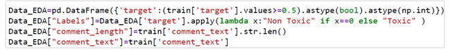
First I am using the following snippet of code to convert target column thresholds to binary labels.

首先，我使用以下代码片段将目标列阈值转换为二进制标签。

现在，让我们绘制分布 (Now, let’s plot the distribution)

We can observe from the plot around 8% of data is toxic and 92% of data is non-toxic.

从图中可以看出，大约8％的数据是有毒的，而92％的数据是无毒的。

Now, let’s check unique and repeated comments in “comment_text” column also check of duplicate rows in the dataset

现在，让我们在“ comment_text”列中检查唯一且重复的注释，并检查数据集中的重复行

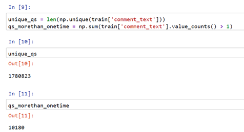
From the above snippet, we got there are 1780823 comments that are unique and 10180 comments are reaping more than once.

从上面的代码片段中，我们得到了1780823条独特的评论，并且10180条评论获得了不止一次的收益。

So we can see in the above snippet there are no duplicate rows in the entire dataset.

因此，我们可以在上面的代码段中看到整个数据集中没有重复的行。

Let’s Plot box Plot for Non-Toxic and Toxic comments based on their lengths

让我们根据它们的长度在方框图中绘制无毒和有毒评论

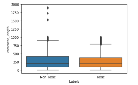
From the above plot, we can observe that most of the points for toxic and non-toxic class comments lengths distributions are overlapping but there are few points in the toxic comments where comment length is more than a thousand words and in the non-toxic comment, we have some point’s are more than 1800 words.

从上图可以看出，有毒和无毒类评论长度分布的大多数点是重叠的，但是有毒评论中评论长度超过一千个单词的点很少，而无毒评论中很少有点，我们有超过1800个单词。

Let’s quickly check the percentile for comment lengths

让我们快速检查百分位数以获取评论长度

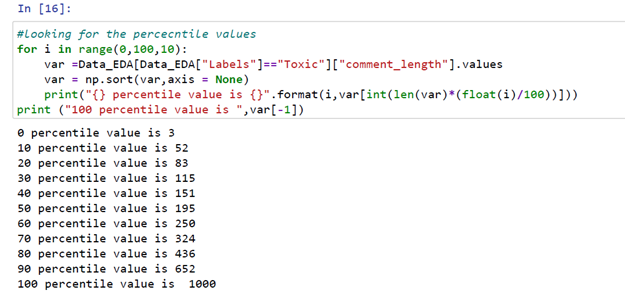
From the above code snippet, we can see the 90th percentile for comment lengths of toxic labels is 652 and the 100th percentile comment length is 1000 words.

从上面的代码片段中，我们可以看到有毒标签的注释长度的第90个百分位数是652，而注释标签的第100个百分位数是1000个单词。

From the above code snippet, we can see the 90th percentile for comment lengths of non-toxic labels is 755 and the 100th percentile comment length is 1956 words.

从上面的代码片段中，我们可以看到无毒标签注释长度的第90个百分位数是755，而注释标签长度的第100个百分位数是1956个单词。

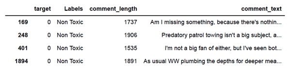
We can easily print some of the comments for which comment has more than 1300 words.

我们可以轻松地打印一些注释，这些注释的注释超过1300个单词。

Let’s plot Word cloud for Toxic and Non-Toxic comments

让我们为有毒和无毒评论绘制词云

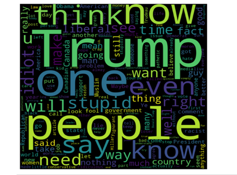
In the above plot, we can see words like trump, stupid, ignorant, people, idiot used in toxic comments with high frequency.

在上面的情节中，我们可以看到诸如特朗普，愚蠢，无知，人，白痴之类的词频繁用于有毒评论。

In the above plot, we can see there are no negative words with the high frequency used in non-toxic comments.

在上图中，我们可以看到在无毒评论中没有使用高频的否定词。

基本特征提取 (Basic Feature Extraction)

Let us now construct a few features for our classical models:

现在让我们为经典模型构造一些功能：

• total_length = length of comment

  total_length =评论长度

• capitals = number of capitals in comment

  大写 =评论中的大写数量

• caps_vs_length = (number of capitals in comment)

  caps_vs_length =(注释中的大写字母数)

• num_exclamation_marks = num exclamation marks

  num_exclamation_marks =惊叹号

• num_question_marks = num question marks

  num_question_marks = num个问号

• num_punctuation = Number of num punctuation

  num_punctuation =标点符号数

• num_symbols = Number of symbols (@, #, $, %, ^, &, *, ~)

  num_symbols =符号数(@，＃，$，％，^，＆，*，〜)

• num_words = Total numer of words

  num_words =单词总数

• num_unique_words = Number unique words

  num_unique_words =唯一字数

• words_vs_unique = number of unique words/number of words

  words_vs_unique =唯一单词数/单词数

• num_smilies = number of smilies

  num_smilies =表情符号数

• word_density = taking average of each word density within the comment

  word_density =取评论中每个单词密度的平均值

• num_stopWords = number of Stopwords in comment

  num_stopWords =注释中停用词的数量

• num_nonStopWords = number of non Stopwords in comment

  num_nonStopWords =注释中非停用词的数量

• num_nonStopWords_density = (num stop words)/(num stop words + num non stop words)

  num_nonStopWords_density =(停止词数)/(停止词数+非停止词数)

• num_stopWords_density = (num non stop words)/(num stop words + num non stop words)

  num_stopWords_density =(num个非终止词)/(num个非终止词+ num个非终止词)

To check the implementation of these features you can check my EDA notebook.

要检查这些功能的实现，可以检查我的EDA笔记本 。

After the implementation of these features let’s check the correlation of extracted feature with target and some of the other features form the dataset.

在实现这些特征之后，让我们检查提取的特征与目标之间的相关性，以及其他一些形成数据集的特征。

So for correlation first I implemented the person correlation of extracted features with some of the features from the dataset and plotted the following the seaborn heatmap plot.

因此，对于关联性，我首先将提取的特征与数据集中的某些特征进行人际关联，然后绘制以下seaborn热图图。

From the above plot, we can observe some good correlations between extracted features and existing features, for example, there is a high positive correlation between target and num_explation_marks, high negative correlation between num_stopWords and funny comments and we can see there are lots of features where there is no correlation between them, for example, num_stopWords with Wow comments and sad comments with num_smilies.

从上面的图中可以看出，提取的特征与现有特征之间存在良好的相关性，例如，目标和num_explation_marks之间的正相关性很高，num_stopWords和有趣的注释之间的负相关性很高，并且可以看到很多特征它们之间没有关联，例如，带有Wow注释的num_stopWords和带有num_smilies的悲伤注释。

功能选择 (Feature selection)

I applied some feature selection methods on extracted features like Filter Method, Wrapper Method, and Embedded Method by following this blog.

通过关注此博客 ，我对提取的特征(例如过滤器方法，包装器方法和嵌入式方法)应用了一些特征选择方法。

Filter Method: In this method, we just filter and select only a subset of relevant features, and filtering is done using the Pearson correlation.

过滤方法 ：在这种方法中，我们仅过滤并选择相关特征的子集，然后使用Pearson相关进行过滤。

Wrapper Method: In this method, we have to use one machine learning model and will evaluate features based on the performance of the selected features. This is an iterative process but better accurate than the filter method. It could be implemented in two ways.

包装器方法：在这种方法中，我们必须使用一种机器学习模型，并将基于所选功能的性能评估功能。 这是一个迭代过程，但比过滤方法更准确。 它可以通过两种方式实现。

1. Backward Elimination: First we feed all the features to the model and evaluate its performance then we eliminate worst-performing features one by one till we get some good relevant performance. It uses pvalue as a performance metric.

1. 向后消除 ：首先，我们将所有特征馈入模型并评估其性能，然后逐一消除性能最差的特征，直到获得良好的相关性能。 它使用pvalue作为性能指标。

2. RFE (Recursive Feature Elimination): In this method, we recursively remove features and build the model on the remaining features. It uses an accuracy metric to rank the feature according to their importance.

2. RFE(递归特征消除) ：在这种方法中，我们递归除去特征，并在其余特征上构建模型。 它使用精度度量根据其重要性对特征进行排名。

Embedded Method: It is one of the methods commonly used by regularization methods that penalize a feature-based n given coefficient threshold of the feature.

嵌入式方法 ：这是正则化方法常用的方法之一，它惩罚基于特征的n个给定特征阈值。

I followed the implantation from this blog and used the Lasso regularization. If the feature is irrelevant, lasso penalizes its coefficient and make it 0. Hence the features with coefficient = 0 are removed and the rest is taken.

我跟踪了此博客中的植入内容，并使用了Lasso正则化。 如果特征不相关，套索将对其系数进行惩罚并将其设为0。因此，系数为0的特征将被删除，其余部分将被采用。

To understand these methods and its implementation more briefly please check this blog.

要更简短地了解这些方法及其实现，请查看此博客。

After implementing all the methods of feature selection I selected the results of the Embedded Method and will include selected features in our training.

实施所有特征选择方法后，我选择了嵌入式方法的结果，并将在我们的培训中包括选定的特征。

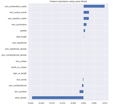
Embedded method mark the following features as unimportant

嵌入式方法将以下功能标记为不重要

1. caps_vs_length

1. caps_vs_length

2. words_vs_unique

2. words_vs_unique

3. num_smilies

3. num_smilies

4. num_nonStopWords_density

4. num_nonStopWords_density

5. num_stopWords_density

5. num_stopWords_density

I plotted some of the selected extracted features as the following plots:

我绘制了一些选定的提取特征，如下图所示：

EDA分析摘要： (Summary of EDA analysis:)

1. The number of Toxic comments is less than Non Toxic comments i.e. 8 percent of toxic 92 percent of non-toxic.

1.有毒评论的数量少于无毒评论，即有毒评论的8％和无毒评论的92％。

2. We printed the percentile values of length of comments and observed the 90th percentile value is 652 for the Toxic and 90th percentile value is 755 for non-Toxic. We also checked there are 7 comments with length more than 1300 and all are non-toxic.

2.我们打印了注释长度的百分位值，观察到有毒的第90个百分位值为652，无毒的第90个百分位值为755。 我们还检查了7条评论，这些评论的长度超过1300，并且均为无毒。

3. We created some text features and plotted the correlation table with Target and Identities Features. We also plotted the correlation table between extracted features Vs extracted features, to check correlation among them.

3.我们创建了一些文本特征，并绘制了带有目标和身份特征的关联表。 我们还绘制了提取特征与提取特征之间的相关表，以检查它们之间的相关性。

4. We applied some feature selection methods and used the results of Embedded Method where out of 16 we selected 11 as relevant features.

4.我们应用了一些特征选择方法，并使用Embedded Method的结果，在16种方法中，我们选择了11种作为相关特征。

5. We plotted the Villon and Density plot for some of the extracted features with target labels.

5.我们绘制了一些带有目标标签的特征的Villon和密度图。

6. We plotted Word cloud for Toxic and Non-Toxic comments and observed some words which are frequently used in Toxic comments.

6.我们绘制了有毒和无毒评论的词云，并观察了有毒评论中经常使用的一些单词。

现在让我们对数据进行一些基本的预处理 (Now let’s do some basic pre-processing on our data)

Checking for NULL values

检查NULL值

From the above snippet, we can observe there is a lot of identity numerical features with lots of null values and there are no null values in comment text feature. Identity numerical features values are thresholds between 0 to1 along with target columns.

从上面的代码片段中，我们可以观察到有很多带有大量空值的标识数字特征，并且注释文本特征中没有空值。 身份数字特征值与目标列一起是介于0到1之间的阈值。

So, I converted the identity features along with the target column as Boolean features as mentioned in competition. Values greater than equal to 0.5 will be marked as True and other than that as False (null values now become False).

因此，我将身份特征与目标列一起转换为竞赛中提到的布尔特征。 大于等于0.5的值将被标记为True，而不是False(空值现在变为False)。

In the below snippet I selected few Identity features for our model's evaluation and converting them to Boolean features along with the target column.

在下面的代码段中，我为模型的评估选择了一些Identity功能，并将其与目标列一起转换为Boolean功能。

As the target column is binary now our data is ready for binary classification models.

由于目标列为二进制，因此我们的数据已准备好用于二进制分类模型。

Now I split the data into Train and Test in 80:20 ratio:

现在，我将数据按80:20的比例分为训练和测试：

For text pre-processing, I am using the following function in which I am implementing

对于文本预处理，我使用以下函数，在其中实现

1. Tokenization

1. 标记化

2. Lemmatization

2. 合法化

3. Stop words removal

3.停止单词删除

4. Applying Regex to remove all non-words token and keeping all special symbols that are commonly used in comments.

4.应用正则表达式删除所有非单词标记，并保留注释中常用的所有特殊符号。

使用Tf Idf矢量化文本 (Vectorizing Text with Tf Idf Vectorize)

As models can’t understand text directly, we have to vectorize our data. So to vectorize our data I selected TfIdf.

由于模型无法直接理解文本，因此我们必须对数据进行矢量化处理。 因此，为了矢量化数据，我选择了TfIdf。

To understand TfIdf and its implementation in python briefly you can check this blog.

要简要了解TfIdf及其在python中的实现，您可以查看此博客。

So, first, we are applying TfIdf on our train data with maximum features as 10000.

因此，首先，我们将TfIdf应用于最大特征为10000的火车数据。

In TfIdf I got the scores for all tokens based on term frequency and inverse document frequency.

在TfIdf中，我根据术语频率和文档反向频率获得了所有令牌的分数。

Higher the score more weightage of the token.

分数越高，令牌的权重越大。

In the following snippet, I collected the tokens along with the TfIdf score in tuples and stored all sorted tuples on the list.

在以下代码段中，我将标记和TfIdf分数一起收集在元组中，并将所有排序后的元组存储在列表中。

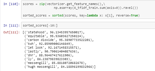
Now based on the scores I selected 150 as threshold and now I will collect all tokens from TfIdf with score greater than 150.

现在基于分数，我选择150作为阈值，现在我将从TfIdf收集分数大于150的所有令牌。

In the following function, I am removing all tokens having a TfIdf score of less than 150.

在以下功能中，我将删除所有TfIdf得分小于150的令牌。

数值特征的标准化 (Standardization of numerical features)

To normalize the extracted numerical features I am using sklearn’s StandardScaler which will standardize the numerical features.

为了标准化提取的数字特征，我使用了sklearn的StandardScaler ，它将标准化数字特征。

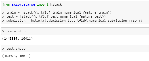
As I pre-processed the numerical extracted features and text feature lets now stack them using scipy’s hstack as follows:

在预处理数字提取功能和文本功能之后，现在使用scipy的 hstack对其进行堆叠，如下所示：

Now our data is ready so let’s start implementing some classical models on it.

现在我们的数据已经准备就绪，让我们开始在其上实现一些经典模型。

经典款 ： (Classical models:)

In this section I will show you some Classical Machine Learning implementation, to check the implementation of all the classical models you can check my notebook.

在本节中，我将向您展示一些经典机器学习实现，以检查所有经典模型的实现，您可以检查我的笔记本。

逻辑回归： (Logistic Regression:)

Logistic Regression one of the popular classification problems. There is a lot of applications that can be applied using a logistic regression classifier for binary classification problems like spam email filter detection, online transaction fraud or not, etc. Now I will apply logistic regression on the pre-processed stacked data.

Logistic回归是流行的分类问题之一。 有很多应用程序可以使用逻辑回归分类器来解决二进制分类问题，例如垃圾邮件过滤器检测，是否进行在线交易欺诈等。现在，我将逻辑回归应用于预处理的堆叠数据。

To know more about logistic regression you can check this blog.

要了解有关逻辑回归的更多信息，可以查看此博客。

In the below snippet you can see I am using sklearn’s GridsearchCV to tune the hyperparameters, I choose value 4 for k cross-validation. Cross validations basically used to evaluate trained models with the different values of hyperparameters.

在下面的代码段中，您可以看到我正在使用sklearn的GridsearchCV调整超参数，我为k交叉验证选择了值4。 交叉验证基本上用于评估具有不同超参数值的训练模型。

I am using different values of alpha’s get the best score. For alpha value 0.0001 I am getting the best score on CV based on GridSearchCV results.

我正在使用不同的alpha值来获得最佳分数。 对于alpha值0.0001，基于GridSearchCV结果，我在CV上获得了最高分。

Next, I trained a logistic regression model with the selected hyperparameter values on trained data, then I used the trained model to predict probabilities on test data.

接下来，我在训练后的数据上使用选定的超参数值训练了逻辑回归模型，然后使用训练后的模型来预测测试数据的概率。

Now I passed the data frame containing Identities columns along with logistic regression probability scores to Evaluation metric function.

现在，我将包含“身份”列的数据框以及逻辑回归概率分数传递给“评估”度量功能。

You can see the complete implantation of the evaluation metric in this Kaggle notebook.

您可以在此 Kaggle笔记本中看到评估指标的完整植入。

Evaluation metric score on test data: 0.57022

测试数据的评估指标得分： 0.57022

On preprocessing text and numerical features on competition’s train data I preprocessed the submission data as well. Now using the trained model I got probability scores for Submission data as well. Now I prepared submission.csv as mentioned in the competition.

在对比赛火车数据的文本和数字特征进行预处理时，我也对提交数据进行了预处理。 现在，使用经过训练的模型，我也获得了提交数据的概率分数。 现在，我准备了竞赛中提到的submit.csv 。

On submitting the submission.csv I got Kaggle score of 0.57187

提交submitt.csv时，我获得Kaggle得分0.57187

Now following the same procedure, I trained all classical models. Please check the following table for the scores of all classification models I implemented.

现在按照相同的步骤，我训练了所有经典模型。 请检查下表，了解我实施的所有分类模型的得分。

So, the XGB classifier gives the best Evaluation metric and test score among all Classical models.

因此，XGB分类器可在所有经典模型中提供最佳的评估指标和测试分数。

Please check part 2 of this project’s blog which explains the deep learning implementations and deployment function of this problem. You can check the implementation of EDA and classical machine learning models notebook on my Github repository.

请检查 该项目博客的 第2部分 ，该博客解释了该问题的深度学习实现和部署功能。 您可以在我的 Github存储库中 检查EDA和经典机器学习模型笔记本的实现 。

未来的工作 (Future work)

Can apply deep learning architectures which can improve the model performance.

可以应用可以改善模型性能的深度学习架构。

1. https://www.kaggle.com/c/jigsaw-unintended-bias-in-toxicity-classification

   https://www.kaggle.com/c/jigsaw-unintended-bias-in-toxicity-classification

2. https://www.kaggle.com/nz0722/simple-eda-text-preprocessing-jigsaw

   https://www.kaggle.com/nz0722/simple-eda-text-preprocessing-jigsaw

3. Paper provided by Conversation AI team explaining the problem and metric briefly https://arxiv.org/abs/1903.04561

   会话AI团队提供的论文简要说明了问题和指标https://arxiv.org/abs/1903.04561

4. https://www.appliedaicourse.com/

   https://www.appliedaicourse.com/

5. https://towardsdatascience.com/feature-selection-with-pandas-e3690ad8504b

   https://towardsdatascience.com/feature-selection-with-pandas-e3690ad8504b