图深度学习-第1部分
有关深层学习的FAU讲义 (FAU LECTURE NOTES ON DEEP LEARNING)
These are the lecture notes for FAU’s YouTube Lecture “Deep Learning”. This is a full transcript of the lecture video & matching slides. We hope, you enjoy this as much as the videos. Of course, this transcript was created with deep learning techniques largely automatically and only minor manual modifications were performed. Try it yourself! If you spot mistakes, please let us know!
这些是FAU YouTube讲座“ 深度学习 ”的 讲义 。 这是演讲视频和匹配幻灯片的完整记录。 我们希望您喜欢这些视频。 当然,此成绩单是使用深度学习技术自动创建的,并且仅进行了较小的手动修改。 自己尝试! 如果发现错误,请告诉我们!
导航 (Navigation)
Previous Lecture / Watch this Video / Top Level / Next Lecture
上一个讲座 / 观看此视频 / 顶级 / 下一个讲座

Welcome back to deep learning! So today, we want to look a bit into how to process graphs and we will talk a bit about graph convolutions. So let’s see what I have here for you. Topic today will be an introduction to graph deep learning.
欢迎回到深度学习! 因此,今天,我们想研究一下如何处理图形,并讨论图形卷积。 因此,让我们看看我在这里为您提供的服务。 今天的主题将是图深度学习的介绍。

Well, what’s graph deep learning? You could say this is a graph, right? We know that from math that we can plot graphs. But this is not what we’re going to talk about today. Also, you could say a graph is like a plot like this one. But these are also not the plots that we want to talk about today. So is it Steffi Graf? No, we are also not talking about Steffi Graf. So what we actually want to look at are more things like this like diagrams that can be connected with different nodes and edges.
那么,什么是图深度学习? 您可以说这是一个图,对吗? 从数学知道,我们可以绘制图形。 但这不是我们今天要谈论的。 此外,您可以说图形就像这样的图形。 但是,这些也不是我们今天要谈论的情节。 那是Steffi Graf吗? 不,我们也没有在谈论Steffi Graf。 因此,我们实际上要看的是更多类似图的东西,它们可以与不同的节点和边连接。

A computer scientist thinks of a graph as a set of nodes and they are connected through edges. So this is the kind of graph that we want to talk about today. For a mathematician, a graph is a manifold, but a discrete one.
计算机科学家将图视为一组节点,并且它们通过边连接。 这就是我们今天要讨论的图表。 对于数学家来说,图是流形,但是离散的。

Now, how would you define a convolution? On euclidean space, well both for computer scientists and mathematicians this is too easy. So this is the discrete convolution which is essentially just a sum. We remember we had many of those discrete convolutions when we are setting up the kernels for our convolutional deep models. In the continuous form, it actually takes the following form: It’s essentially an integral that is computed over the entire space and I brought an example here. So if you want to convolve two Gaussian curves, then you essentially move them over each other multiply at each point and sum them up. Of course, the convolution of two Gaussians is a Gaussian again so this is also easy.
现在,您将如何定义卷积? 在欧几里德空间上,对于计算机科学家和数学家来说,这都太容易了。 因此,这就是离散卷积,本质上只是一个和。 我们记得在为卷积深度模型设置内核时,曾有很多离散卷积。 在连续形式中,它实际上采取以下形式:它本质上是一个在整个空间中计算的整数,在此我举了一个例子。 因此,如果要对两条高斯曲线进行卷积,则实际上是将它们在每个点上彼此相乘,然后求和。 当然,两个高斯的卷积又是高斯,因此这也很容易。

How would you define a convolution on graphs? Now, the computer scientist thinks really hard but … What the heck! Well, the mathematician knows that we can use Laplace transforms in order to describe convolutions and therefore we look into the laplacian that is here given as the divergence of the gradient. So in math, we can deal with these things more easily.
您如何定义图的卷积? 现在,计算机科学家真的很努力地思考,但是……这太糟糕了! 好吧,数学家知道我们可以使用拉普拉斯变换来描述卷积,因此我们研究了拉普拉斯算子,这里给出的是梯度散度。 因此,在数学上,我们可以更轻松地处理这些事情。

This then brings us to this manifold idea. We know how to convolve manifolds, we can discretize convolutions, and this means that we know how to convolve graphs.
然后,这使我们想到了这个多方面的想法。 我们知道如何对流形进行卷积,我们可以使卷积离散化,这意味着我们知道如何对图进行卷积。

So, let’s diffuse some heat! We know that we can describe Newton’s law of cooling as the following equation. We also know that the development over time can be described with the Laplacian. So, f(x,t) is then the amount of heat at point x at time t. Then, you need to have an initial heat distribution. So, you need to know how the heat is in the initial state. Then, you can use the Laplacian in order to express how the system behaves over time. Here, you can see that this is essentially the difference between f(x) and the average of f on an infinite decimal small sphere around x.
因此,让我们散发一些热量! 我们知道我们可以将牛顿冷却定律描述为以下等式。 我们也知道,随着时间的发展可以用拉普拉斯人来描述。 因此,f(x,t)就是时间t处x点的热量。 然后,您需要具有初始热分布。 因此,您需要知道热量在初始状态如何。 然后,您可以使用拉普拉斯算子来表达系统随着时间的变化。 在这里,您可以看到,这实际上是f(x)与x周围无穷小十进制小球体上f的平均值之间的差。

Now, how do we express the Laplacian in discrete form? Well, that’s the difference between f(x) and the average of f on an infinitesimal sphere around x. So, the smallest step that we can do is actually connect the current node with its neighbors. So, we can express the Laplacian as a weighted sum over the edge weights a subscript i and j. This is then the difference of our center node f subscript i minus f subscript j and we divide the whole thing by the number of connections that actually are incoming into f subscript i. This is going to be given as d subscript i.
现在,我们如何以离散形式表示拉普拉斯算子? 好吧,这就是f(x)与x周围无穷小球面上f的平均值之间的差。 因此,我们可以做的最小步骤是实际上将当前节点与其邻居连接起来。 因此,我们可以将拉普拉斯算子表示为边缘权重下标i和j的加权和。 这就是我们的中心节点f下标i减去f下标j的差,我们将整个事物除以实际进入f下标i的连接数。 这将以d下标i给出。

Now is there another way of expressing this? Well, yes. We can do this if we look at an example graph here. So, we have the nodes 1, 2, 3, 4, 5, and 6. We can now compute the Laplacian matrix using the matrix D. D is now simply the number of incoming connections into the respective nodes. So, we can see that Node 1 has two incoming connections, Node 2 has three, Node 3 has two, Node 4 has three, and Node 5 also has three, Node 6 has only one incoming connection. What we else need is the matrix A. That’s the adjacency matrix. So here, we have a 1 for every node that is connected with a different node and you can see it can be expressed with the above matrix now. We can take the two and compute the Laplacian as D minus A. We simply element-wise subtract the two to get our Laplacian matrix. This is nice.
现在还有另一种表达方式吗? 嗯,是。 如果我们在这里查看示例图,则可以执行此操作。 因此,我们有节点1、2、3、4、5和6。现在,我们可以使用矩阵D计算拉普拉斯矩阵。 D现在只是进入各个节点的传入连接数。 因此,我们可以看到节点1具有两个传入连接,节点2具有三个进入节点,节点3具有两个,节点4具有三个,节点5也具有三个,节点6仅具有一个传入连接。 我们还需要矩阵A。 这就是邻接矩阵。 因此,在这里,与不同节点连接的每个节点都有一个1,您现在可以看到它可以用上述矩阵表示。 我们可以将两者取和,将Laplacian计算为D减去A。 我们简单地逐元素相减两个即可得到拉普拉斯矩阵。 很好

We can see that the Laplacian is an N times N matrix and it’s describing a graph or subgraph consisting of N nodes. D is also an N times N matrix and it’s called the degree matrix and describes the number of edges connected to each node. A is also an N times N matrix and it’s the adjacency matrix that describes the connectivity of the graph. So for a directed graph, our graph Laplacian matrix is not symmetric positive definite. So, we need to normalize it in order to get a symmetric version. This can be done in the following way: We start with the original Laplacian matrix. We know that D is simply a diagonal matrix. So, we can compute the inverse square root and multiply it from the left-hand side and right-hand side. Then, we can plug in the original definition and you see that we can rearrange this a little bit. We can then write the symmetrized version as the unity matrix minus D. Here, we apply again element-wise the inverse and the square root times A times the same matrix. So this is very interesting, right? We can always get the symmetrized version of this matrix even for directed graphs.
我们可以看到拉普拉斯算子是N乘N的矩阵,它描述的是由N个节点组成的图或子图。 D也是N乘N的矩阵,它称为度矩阵,描述了连接到每个节点的边的数量。 A也是N乘N的矩阵,它是描述图的连通性的邻接矩阵。 因此对于有向图,我们的图拉普拉斯矩阵不是对称正定的。 因此,我们需要对其进行规范化以获得对称版本。 这可以通过以下方式完成:我们从原始的拉普拉斯矩阵开始。 我们知道D只是对角矩阵。 因此,我们可以计算平方根的倒数,并从左侧和右侧将其相乘。 然后,我们可以插入原始定义,您会看到我们可以重新排列一下。 然后,我们可以将对称形式写为单位矩阵减去D。 在这里,我们再次按元素方式应用逆矩阵和平方根时间A乘同一矩阵。 所以这很有趣,对吗? 即使对于有向图,我们也总是可以获得该矩阵的对称形式。
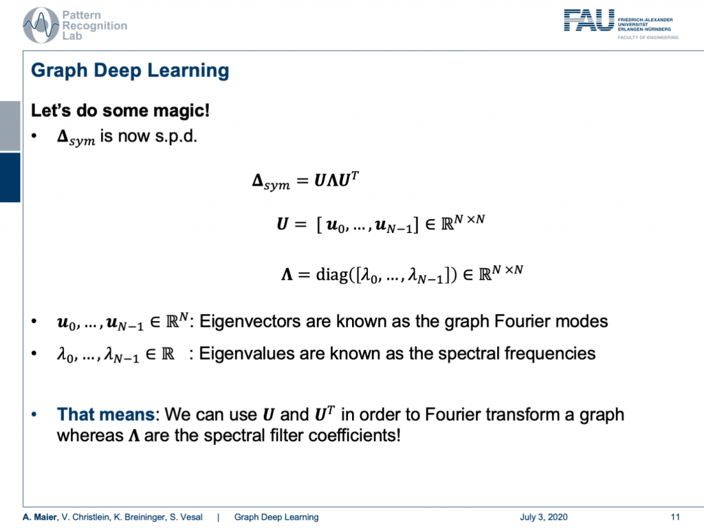
Now, we are interested in how to use this actually. We can do some magic and the magic now is if our matrix is symmetric positive definite, then the matrix can be decomposed into eigenvectors and eigenvalues. Here, we see that all the eigenvectors are assembled in U and the eigenvalues are on this diagonal matrix Λ. Now, these eigenvectors are known as the graph Fourier modes. The eigenvalues are known as spectral frequencies. This means that we can use U and Utranspose in order to Fourier transform a graph and our Λ are the spectral filter coefficients. So, we can transform a graph into a spectral representation and look at its spectral properties.
现在,我们对如何实际使用它感兴趣。 我们可以做一些魔术,现在的魔术是,如果我们的矩阵是对称正定的,那么矩阵可以分解为特征向量和特征值。 在这里,我们看到所有特征向量都以U组合,并且特征值在此对角矩阵Λ上 。 现在,这些特征向量被称为图傅立叶模式。 特征值称为频谱频率。 这意味着我们可以使用U和U转置来对图进行傅立叶变换,而我们的Λ是频谱滤波器系数。 因此,我们可以将图形转换成光谱表示形式,并查看其光谱特性。

Let’s continue with our matrix. Now, let x be some signal, a scalar for every node. Then, we can use the Laplacian’s eigenvectors to define its Fourier transform. This then is simply x hat and x hat can be expressed as U transposed times x. Of course, you can also invert this. This is simply done by applying U. So, we can also find for any set of coefficients that are describing properties of the nodes, the respective spectral representation. Now, we can also describe a convolution with a filter in the spectral domain. So, we express the convolution using a Fourier representation and therefore we bring g and x into Fourier domain, multiply the two and compute the inverse Fourier transform. So, we know that from signal processing that we can also do this in traditional signals.
让我们继续我们的矩阵。 现在,让x为某个信号,每个节点的标量。 然后,我们可以使用拉普拉斯特征向量来定义其傅立叶变换。 那么这就是x hat, x hat可以表示为U换位乘以x 。 当然,您也可以将其反转。 只需通过应用U即可完成。 因此,我们还可以找到描述节点属性的任何系数集,相应的频谱表示形式。 现在,我们还可以描述在频谱域中使用滤波器的卷积。 因此,我们使用傅立叶表示来表示卷积,因此将g和x带入傅立叶域,将二者相乘并计算傅立叶逆变换。 因此,我们知道从信号处理中我们也可以在传统信号中做到这一点。

Now, let’s construct a filter. This filter is composed of a k-th order polynomial of Laplacians with coefficients θ subscript i. They are simply real numbers. So, we can now find this kind of polynomial that is a polynomial with respect to the spectral coefficients and it’s linear in the coefficients θ. This is essentially just a sum over the polynomials. So now, we can use that and use this filter in order to perform our convolution. We essentially have to multiply in the same way as we did before. So, we have the signal, we apply the Fourier transform, then we apply our convolution using our polynomial, and then we do the inverse Fourier transform. So, this would be how we would apply this filter to a new signal. And now, what? Well, we can convolve x now using the laplacian as we adapt our filter coefficients θ. But U is actually really heavy. Remember we can’t use the trick of a fast Fourier transform here. So, it’s always a full matrix multiplication and this might be very heavy to compute if you want to express your convolutions in this type of format. But what if I told you that a clever choice of polynomials cancels out U entirely?
现在,让我们构造一个过滤器。 这个滤波器由拉普拉斯算子的第k阶多项式具有系数θ下标i的。 它们只是实数。 因此,我们现在可以找到这种多项式,它是关于频谱系数的多项式,并且在系数θ中是线性的。 这实际上只是多项式的和。 因此,现在,我们可以使用它并使用此过滤器来执行卷积。 本质上,我们必须以与以前相同的方式进行乘法。 因此,我们得到信号,应用傅立叶变换,然后使用多项式应用卷积,然后进行傅立叶逆变换。 因此,这就是我们将滤波器应用于新信号的方式。 现在呢? 好了,我们现在可以使用拉普拉斯算子对x进行卷积,因为我们可以调整滤波器系数θ 。 但是, U实际上真的很重。 请记住,这里我们不能使用快速傅立叶变换的技巧。 因此,它始终是一个完整的矩阵乘法,如果您想以这种格式表示卷积,那么计算起来可能会很繁重。 但是,如果我告诉您,多项式的明智选择会完全抵消U ?
Well, this is what we will discuss in the next session on deep learning. So, thank you very much for listening so far and see you in the next video. Bye-bye!
好吧,这就是我们将在下一届深度学习会议上讨论的内容。 因此,非常感谢您到目前为止的收听,并在下一个视频中与您相见。 再见!
If you liked this post, you can find more essays here, more educational material on Machine Learning here, or have a look at our Deep LearningLecture. I would also appreciate a follow on YouTube, Twitter, Facebook, or LinkedIn in case you want to be informed about more essays, videos, and research in the future. This article is released under the Creative Commons 4.0 Attribution License and can be reprinted and modified if referenced. If you are interested in generating transcripts from video lectures try AutoBlog.
如果你喜欢这篇文章,你可以找到这里更多的文章 ,更多的教育材料,机器学习在这里 ,或看看我们的深入 学习 讲座 。 如果您希望将来了解更多文章,视频和研究信息,也欢迎关注YouTube , Twitter , Facebook或LinkedIn 。 本文是根据知识共享4.0署名许可发布的 ,如果引用,可以重新打印和修改。 如果您对从视频讲座中生成成绩单感兴趣,请尝试使用AutoBlog 。
谢谢 (Thanks)
Many thanks to the great introduction by Michael Bronstein on MISS 2018 and special thanks to Florian Thamm for preparing this set of slides.
非常感谢Michael Bronstein在MISS 2018上的精彩介绍,特别感谢Florian Thamm准备了这组幻灯片。
翻译自: https://towardsdatascience.com/graph-deep-learning-part-1-e9652e5c4681
http://www.taodudu.cc/news/show-997484.html
相关文章:
- 项目经济规模的估算方法_估算英国退欧的经济影响
- 机器学习 量子_量子机器学习:神经网络学习
- 爬虫神经网络_股市筛选和分析:在投资中使用网络爬虫,神经网络和回归分析...
- 双城记s001_双城记! (使用数据讲故事)
- rfm模型分析与客户细分_如何使用基于RFM的细分来确定最佳客户
- 数据仓库项目分析_数据分析项目:仓库库存
- 有没有改期末考试成绩的软件_如果考试成绩没有正常分配怎么办?
- 探索性数据分析(EDA):Python
- 写作工具_4种加快数据科学写作速度的工具
- 大数据(big data)_如何使用Big Query&Data Studio处理和可视化Google Cloud上的财务数据...
- 多元时间序列回归模型_多元时间序列分析和预测:将向量自回归(VAR)模型应用于实际的多元数据集...
- 数据分析和大数据哪个更吃香_处理数据,大数据甚至更大数据的17种策略
- 批梯度下降 随机梯度下降_梯度下降及其变体快速指南
- 生存分析简介:Kaplan-Meier估计器
- 使用r语言做garch模型_使用GARCH估计货币波动率
- 方差偏差权衡_偏差偏差权衡:快速介绍
- 分节符缩写p_p值的缩写是什么?
- 机器学习 预测模型_使用机器学习模型预测心力衰竭的生存时间-第一部分
- Diffie Hellman密钥交换
- linkedin爬虫_您应该在LinkedIn上关注的8个人
- 前置交换机数据交换_我们的数据科学交换所
- 量子相干与量子纠缠_量子分类
- 知识力量_网络分析的力量
- marlin 三角洲_带火花的三角洲湖:什么和为什么?
- eda分析_EDA理论指南
- 简·雅各布斯指数第二部分:测试
- 抑郁症损伤神经细胞吗_使用神经网络探索COVID-19与抑郁症之间的联系
- 如何开始使用任何类型的数据? - 第1部分
- 机器学习图像源代码_使用带有代码的机器学习进行快速房地产图像分类
- COVID-19和世界幸福报告数据告诉我们什么?
图深度学习-第1部分相关推荐
- 想入门图深度学习?这篇55页的教程帮你理清楚了脉络
选自arXiv 作者:David Bacciu等 机器之心编译 意大利比萨大学的研究者发表论文,介绍了图深度学习领域的主要概念.思想和应用.与其他论文不同的是,这篇论文更像一份入门教程,既适合初学者作 ...
- 【NAACL2021】Graph4NLP:图深度学习自然语言处理(附ppt)
来源:专知本文约1500字,建议阅读5分钟 最新图深度学习在自然语言处理应用的概述报告,不可错过! 深度学习已经成为自然语言处理(NLP)研究的主导方法,特别是在大规模语料库中.在自然语言处理任务中, ...
- 图深度学习:成功,挑战以及后面的路
2020-07-07 10:24:07 作者:Michael Bronstein 编译:ronghuaiyang 导读 介绍了图深度学习取得的一些成果,面对的挑战以及后面的发展之路. 图深度学习,也被 ...
- 图深度学习(GraphDL),下一个人工智能算法热点
https://www.toutiao.com/a6641731848772780548/ 2019-01-02 11:11:41 原创: 专知 [导读]最近,DeepMind.Google大脑.MI ...
- 大咖力荐!图深度学习奠基性著作重磅上市 | 送书福利
马耀,汤继良 著 王怡琦,金卫 译 电子工业出版社-博文视点 2021-05-01 ISBN: 9787121394782 定价: 118.00 元 新书推荐 ????今日福利 |关于本书| 本书全面 ...
- 腾讯AI Lab联合清华,港中文长文解析图深度学习的历史、最新进展到应用
本文作者: 腾讯:荣钰.徐挺洋.黄俊洲:清华大学:黄文炳:香港中文大学:程鸿 前言 人工智能领域近几年历经了突飞猛进的发展.图像.视频.游戏博弈.自然语言处理.金融等大数据分析领域都实现了跨越式的进步 ...
- 启动图一键生成工具_一键即运行!清华团队推出图深度学习工具包CogDL v0.1
一行代码命令可以做什么? "一行命令可以实现'一条龙'运行实验." 访问 http://github.com/THUDM/cogdl 一键体验! 近年来,结构化数据的表示学习备受业 ...
- 图深度学习-第2部分
有关深层学习的FAU讲义 (FAU LECTURE NOTES ON DEEP LEARNING) These are the lecture notes for FAU's YouTube Lect ...
- 图深度学习前沿工作汇总与解析
图深度学习除了可以应用于标准图推理任务以外,还广泛应用于推荐.疾病或药物预测.自然语言处理.计算机视觉.交通预测等领域. 可见,基于图的深度学习不仅有助于挖掘现有图数据背后的丰富价值,而且还通过将关系 ...
最新文章
- 前端性能优化之DOM(三)
- Java中 break、continue 和 return三者之间的区别
- centos nginx不是命令_虚拟机下Centos 8.0 安装PHP+Mysql+Nginx
- 分布式Session解决方案_Token + Redis
- sql server management studio性能分析_如何分析一条SQL的性能
- Java生产环境下性能监控与调优详解 第2章 基于JDK命令行工具的监控
- DCI架构是如何解决DDD战术建模缺点的?
- 电商促销海报设计技巧!
- android sdk httppost,android6.0SDK 删除HttpClient的相关类的解决方法
- 1104 LED Test
- laravel框架连接Oracle,laravel5.8(十四)连接oracle数据库
- 基于kl变换的人脸识别_简述几种人脸识别的主要方法
- JAVA ik es_Elasticsearch入门和查询语法分析(ik中文分词)
- Python实用模块(二十四)tenacity
- 软件使用说明书编写格式规范
- Java随笔记录第三章:数组
- 【歪门邪道】Android中如何快速回到主页
- Ubuntu安装Lua
- JavaScript 绝妙的函数:模块模式
- dataframe格式知识点总结