Python计算机视觉:第二章 图像局部描述符
第二章 图像局部描述符
- 2.1 Harris角点检测
- 2.1.2 在图像间寻找对应点
- 2.2 sift描述子
- 2.2.1 兴趣点
- 2.2.2 描述子
- 2.2.3 检测感兴趣点
- 2.2.4 描述子匹配
- 2.3 地理标记图像匹配
- 2.3.1 从Panoramio下载地理标记图像
- 2.3.2 用局部描述子进行匹配
- 2.3.3 可视化接连的图片
这一章主要介绍两种非常典型的、不同的图像描述子,这两种图像描述子的使用将贯穿于本书,并且作为重要的局部特征,它们应用到了很多应用领域,比如创建全景图、增强现实、3维重建等。
2.1 Harris角点检测
Harris角点检测算法是最简单的角点检测方法之一。关于harris算法的原理,可以参阅本书中译本。下面是harris角点检测实例代码。
# -*- coding: utf-8 -*-
from pylab import *
from PIL import Image
from PCV.localdescriptors import harris"""
Example of detecting Harris corner points (Figure 2-1 in the book).
"""# 读入图像
im = array(Image.open('../data/empire.jpg').convert('L'))# 检测harris角点
harrisim = harris.compute_harris_response(im)# Harris响应函数
harrisim1 = 255 - harrisimfigure()
gray()#画出Harris响应图
subplot(141)
imshow(harrisim1)
print harrisim1.shape
axis('off')
axis('equal')threshold = [0.01, 0.05, 0.1]
for i, thres in enumerate(threshold):filtered_coords = harris.get_harris_points(harrisim, 6, thres)subplot(1, 4, i+2)imshow(im)print im.shapeplot([p[1] for p in filtered_coords], [p[0] for p in filtered_coords], '*')axis('off')#原书采用的PCV中PCV harris模块
#harris.plot_harris_points(im, filtered_coords)# plot only 200 strongest
# harris.plot_harris_points(im, filtered_coords[:200])show()
运行上面代码,可得原书P32页的图: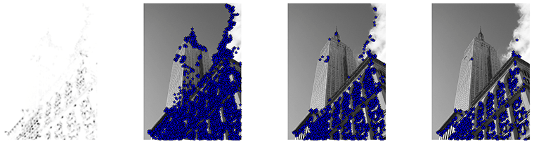 在上面代码中,先代开一幅图像,将其转换成灰度图像,然后计算相响应函数,通过响应值选择角点。最后,将这些检测的角点在原图上显示出来。如果你想对角点检测方法做一个概览,包括想对Harris检测器做些提高或改进,可以参阅WIKI中的例子WIKI.
2.1.2 在图像间寻找对应点
Harris角点检测器可以给出图像中检测到兴趣点,但它并没有提供在图像间对兴趣点进行比较的方法,我们需要在每个角点添加描述子,以及对这些描述子进行比较。关于兴趣点描述子,见本书中译本。下面再现原书P35页中的结果:
# -*- coding: utf-8 -*-
from pylab import *
from PIL import Imagefrom PCV.localdescriptors import harris
from PCV.tools.imtools import imresize"""
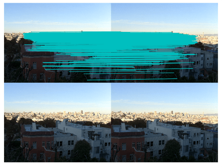
This is the Harris point matching example in Figure 2-2.
"""# Figure 2-2上面的图
#im1 = array(Image.open("../data/crans_1_small.jpg").convert("L"))
#im2= array(Image.open("../data/crans_2_small.jpg").convert("L"))# Figure 2-2下面的图
im1 = array(Image.open("../data/sf_view1.jpg").convert("L"))
im2 = array(Image.open("../data/sf_view2.jpg").convert("L"))# resize加快匹配速度
im1 = imresize(im1, (im1.shape[1]/2, im1.shape[0]/2))
im2 = imresize(im2, (im2.shape[1]/2, im2.shape[0]/2))wid = 5
harrisim = harris.compute_harris_response(im1, 5)
filtered_coords1 = harris.get_harris_points(harrisim, wid+1)
d1 = harris.get_descriptors(im1, filtered_coords1, wid)harrisim = harris.compute_harris_response(im2, 5)
filtered_coords2 = harris.get_harris_points(harrisim, wid+1)
d2 = harris.get_descriptors(im2, filtered_coords2, wid)print 'starting matching'
matches = harris.match_twosided(d1, d2)figure()
gray()
harris.plot_matches(im1, im2, filtered_coords1, filtered_coords2, matches)
show()
运行上面代码,可得下图: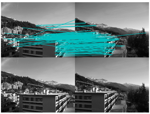 正如你从上图所看到的,这里有很多错配的。近年来,提高特征描述点检测与描述有了很大的发展,在下一节我们会看这其中最好的算法之一——SIFT。
2.2 sift描述子
在过去的十年间,最成功的图像局部描述子之一是尺度不变特征变换(SIFT),它是由David Lowe发明的。SIFT在2004年由Lowe完善并经受住了时间的考验。关于SIFT原理的详细介绍,可以参阅中译本,在WIKI上你可以看一个简要的概览。
2.2.1 兴趣点
2.2.2 描述子
2.2.3 检测感兴趣点
为了计算图像的SIFT特征,我们用开源工具包VLFeat。用Python重新实现SIFT特征提取的全过程不会很高效,而且也超出了本书的范围。VLFeat可以在www.vlfeat.org上下载,它的二进制文件可以用于一些主要的平台。这个库是用C写的,不过我们可以利用它的命令行接口。此外,它还有Matlab接口。下面代码是再现原书P40页的代码:
# -*- coding: utf-8 -*-
from PIL import Image
from pylab import *
from PCV.localdescriptors import sift
from PCV.localdescriptors import harris# 添加中文字体支持
from matplotlib.font_manager import FontProperties
font = FontProperties(fname=r"c:\windows\fonts\SimSun.ttc", size=14)imname = '../data/empire.jpg'
im = array(Image.open(imname).convert('L'))
sift.process_image(imname, 'empire.sift')
l1, d1 = sift.read_features_from_file('empire.sift')figure()
gray()
subplot(131)
sift.plot_features(im, l1, circle=False)
title(u'SIFT特征',fontproperties=font)
subplot(132)
sift.plot_features(im, l1, circle=True)
title(u'用圆圈表示SIFT特征尺度',fontproperties=font)# 检测harris角点
harrisim = harris.compute_harris_response(im)subplot(133)
filtered_coords = harris.get_harris_points(harrisim, 6, 0.1)
imshow(im)
plot([p[1] for p in filtered_coords], [p[0] for p in filtered_coords], '*')
axis('off')
title(u'Harris角点',fontproperties=font)show()
运行上面代码,可得下图: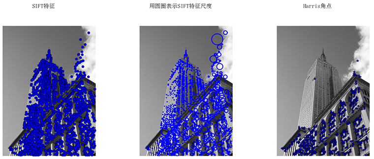 为了将sift和Harris角点进行比较,将Harris角点检测的显示在了图像的最后侧。正如你所看到的,这两种算法选择了不同的坐标。
2.2.4 描述子匹配
from PIL import Image
from pylab import *
import sys
from PCV.localdescriptors import siftif len(sys.argv) >= 3:im1f, im2f = sys.argv[1], sys.argv[2]
else:
# im1f = '../data/sf_view1.jpg'
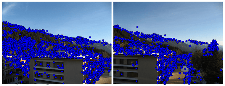
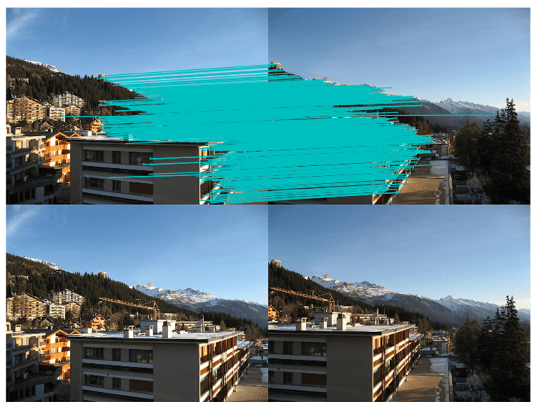
# im2f = '../data/sf_view2.jpg'im1f = '../data/crans_1_small.jpg'im2f = '../data/crans_2_small.jpg'
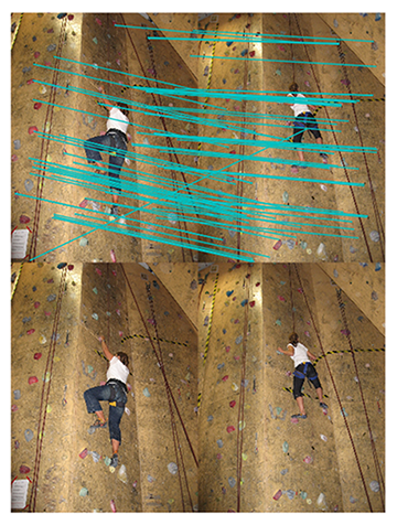
# im1f = '../data/climbing_1_small.jpg'
# im2f = '../data/climbing_2_small.jpg'
im1 = array(Image.open(im1f))
im2 = array(Image.open(im2f))sift.process_image(im1f, 'out_sift_1.txt')
l1, d1 = sift.read_features_from_file('out_sift_1.txt')
figure()
gray()
subplot(121)
sift.plot_features(im1, l1, circle=False)sift.process_image(im2f, 'out_sift_2.txt')
l2, d2 = sift.read_features_from_file('out_sift_2.txt')
subplot(122)
sift.plot_features(im2, l2, circle=False)#matches = sift.match(d1, d2)
matches = sift.match_twosided(d1, d2)
print '{} matches'.format(len(matches.nonzero()[0]))figure()
gray()
sift.plot_matches(im1, im2, l1, l2, matches, show_below=True)
show()
运行上面代码,可得下图: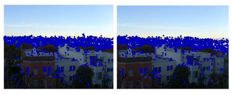
2.3 地理标记图像匹配
在结束本章前,我们看一个用局部描述子对地理标记图像进行匹配的例子。
2.3.1 从Panoramio下载地理标记图像
利用谷歌的图片分享服务Panoramio,可以下载地理标记图像。像很多其他的web服务一样,Panoramio提供了API接口,通过提交HTTP GET请求url:
http://www.panoramio.com/map/get_panoramas.php?order=popularity&set=public&
from=0&to=20&minx=-180&miny=-90&maxx=180&maxy=90&size=medium
上面minx、miny、maxx、maxy定义了获取照片的地理区域。下面代码是获取白宫地理区域的照片实例:
# -*- coding: utf-8 -*-
import json
import os
import urllib
import urlparse
from PCV.tools.imtools import get_imlist
from pylab import *
from PIL import  Image#change the longitude and latitude here
#here is the longitude and latitude for Oriental Pearl
minx = '-77.037564'
maxx = '-77.035564'
miny = '38.896662'
maxy = '38.898662'#number of photos
numfrom = '0'
numto = '20'
url = 'http://www.panoramio.com/map/get_panoramas.php?order=popularity&set=public&from=' + numfrom + '&to=' + numto + '&minx=' + minx + '&miny=' + miny + '&maxx=' + maxx + '&maxy=' + maxy + '&size=medium'#this is the url configured for downloading whitehouse photos. Uncomment this, run and see.
#url = 'http://www.panoramio.com/map/get_panoramas.php?order=popularity&\
#set=public&from=0&to=20&minx=-77.037564&miny=38.896662&\
#maxx=-77.035564&maxy=38.898662&size=medium'c = urllib.urlopen(url)j = json.loads(c.read())
imurls = []
for im in j['photos']:imurls.append(im['photo_file_url'])for url in imurls:image = urllib.URLopener()image.retrieve(url, os.path.basename(urlparse.urlparse(url).path))print 'downloading:', url#显示下载到的20幅图像
figure()
gray()
filelist = get_imlist('./')
for i, imlist in enumerate(filelist):im=Image.open(imlist)subplot(4,5,i+1)imshow(im)axis('off')
show()
译者稍微修改了原书的代码,上面numto是设置下载照片的数目。运行上面代码可在脚本所在的目录下得到下载到的20张图片,代码后面部分为译者所加,用于显示下载到的20幅图像: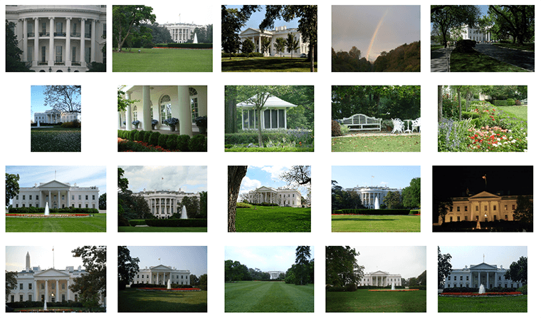 现在我们便可以用这些图片利用局部特征对其进行匹配了。
2.3.2 用局部描述子进行匹配
在下载完上面的图片后,我们便可提取他们的描述子。这里,我们用前面用到的SIFT描述子。
# -*- coding: utf-8 -*-
from pylab import *
from PIL import Image
from PCV.localdescriptors import sift
from PCV.tools import imtools
import pydot""" This is the example graph illustration of matching images from Figure 2-10.
To download the images, see ch2_download_panoramio.py."""#download_path = "panoimages"  # set this to the path where you downloaded the panoramio images
#path = "/FULLPATH/panoimages/"  # path to save thumbnails (pydot needs the full system path)download_path = "F:/dropbox/Dropbox/translation/pcv-notebook/data/panoimages"  # set this to the path where you downloaded the panoramio images
path = "F:/dropbox/Dropbox/translation/pcv-notebook/data/panoimages/"  # path to save thumbnails (pydot needs the full system path)# list of downloaded filenames
imlist = imtools.get_imlist(download_path)
nbr_images = len(imlist)# extract features
featlist = [imname[:-3] + 'sift' for imname in imlist]
for i, imname in enumerate(imlist):sift.process_image(imname, featlist[i])matchscores = zeros((nbr_images, nbr_images))for i in range(nbr_images):for j in range(i, nbr_images):  # only compute upper triangleprint 'comparing ', imlist[i], imlist[j]l1, d1 = sift.read_features_from_file(featlist[i])l2, d2 = sift.read_features_from_file(featlist[j])matches = sift.match_twosided(d1, d2)nbr_matches = sum(matches > 0)print 'number of matches = ', nbr_matchesmatchscores[i, j] = nbr_matches
print "The match scores is: \n", matchscores# copy values
for i in range(nbr_images):for j in range(i + 1, nbr_images):  # no need to copy diagonalmatchscores[j, i] = matchscores[i, j]
上面将两两进行特征匹配后的匹配数保存在matchscores中,最后一部分将矩阵填充完整,它并不是必须的,原因是该“距离度量”矩阵是对称的。运行上面代码,可得到下面的结果:
662 0 0 2 0 0 0 0 1 0 0 1 2 0 3 0 19 1 0 2
0 901 0 1 0 0 0 1 1 0 0 1 0 0 0 0 0 0 1 2
0 0 266 0 0 0 0 0 0 0 0 0 0 1 0 0 0 0 0 0
2 1 0 1481 0 0 2 2 0 0 0 2 2 0 0 0 2 3 2 0
0 0 0 0 1748 0 0 1 0 0 0 0 0 2 0 0 0 0 0 1
0 0 0 0 0 1747 0 0 1 0 0 0 0 0 0 0 0 1 1 0
0 0 0 2 0 0 555 0 0 0 1 4 4 0 2 0 0 5 1 0
0 1 0 2 1 0 0 2206 0 0 0 1 0 0 1 0 2 0 1 1
1 1 0 0 0 1 0 0 629 0 0 0 0 0 0 0 1 0 0 20
0 0 0 0 0 0 0 0 0 829 0 0 1 0 0 0 0 0 0 2
0 0 0 0 0 0 1 0 0 0 1025 0 0 0 0 0 1 1 1 0
1 1 0 2 0 0 4 1 0 0 0 528 5 2 15 0 3 6 0 0
2 0 0 2 0 0 4 0 0 1 0 5 736 1 4 0 3 37 1 0
0 0 1 0 2 0 0 0 0 0 0 2 1 620 1 0 0 1 0 0
3 0 0 0 0 0 2 1 0 0 0 15 4 1 553 0 6 9 1 0
0 0 0 0 0 0 0 0 0 0 0 0 0 0 0 2273 0 1 0 0
19 0 0 2 0 0 0 2 1 0 1 3 3 0 6 0 542 0 0 0
1 0 0 3 0 1 5 0 0 0 1 6 37 1 9 1 0 527 3 0
0 1 0 2 0 1 1 1 0 0 1 0 1 0 1 0 0 3 1139 0
2 2 0 0 1 0 0 1 20 2 0 0 0 0 0 0 0 0 0 499
注意:这里译者为排版美观起见,用的是原书运行的结果,上面代码时间运行的结果跟原书得到的结果是有差异的。
2.3.3 可视化接连的图片
这节我们对上面匹配后的图像进行连接可视化,要做到这样,我们需要在一个图中用边线表示它们之间是相连的。我们采用pydot工具包,它提供了GraphViz graphing库的Python接口。不要担心,它们安装起来很容易。
Pydot很容易使用,下面代码演示创建一个图:
import pydotg = pydot.Dot(graph_type='graph')g.add_node(pydot.Node(str(0), fontcolor='transparent'))
for i in range(5):g.add_node(pydot.Node(str(i + 1)))g.add_edge(pydot.Edge(str(0), str(i + 1)))for j in range(5):g.add_node(pydot.Node(str(j + 1) + '0' + str(i + 1)))g.add_edge(pydot.Edge(str(j + 1) + '0' + str(i + 1), str(j + 1)))
g.write_png('../images/ch02/ch02_fig2-9_graph.png', prog='neato')
运行上面代码,在images/ch02/下生成一幅名字为ch02fig2-9graph的图,如下所示: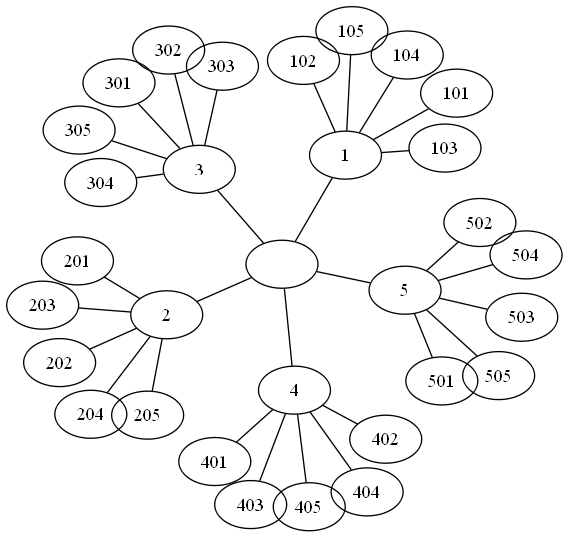 现在,我们回到那个地理图像的例子,我们同样将匹配后对其进行可视化。为了是得到的可视化结果比较好看,我们对每幅图像用100*100的缩略图缩放它们。
# -*- coding: utf-8 -*-
from pylab import *
from PIL import Image
from PCV.localdescriptors import sift
from PCV.tools import imtools
import pydot""" This is the example graph illustration of matching images from Figure 2-10.
To download the images, see ch2_download_panoramio.py."""#download_path = "panoimages"  # set this to the path where you downloaded the panoramio images
#path = "/FULLPATH/panoimages/"  # path to save thumbnails (pydot needs the full system path)download_path = "F:/dropbox/Dropbox/translation/pcv-notebook/data/panoimages"  # set this to the path where you downloaded the panoramio images
path = "F:/dropbox/Dropbox/translation/pcv-notebook/data/panoimages/"  # path to save thumbnails (pydot needs the full system path)# list of downloaded filenames
imlist = imtools.get_imlist(download_path)
nbr_images = len(imlist)# extract features
featlist = [imname[:-3] + 'sift' for imname in imlist]
for i, imname in enumerate(imlist):sift.process_image(imname, featlist[i])matchscores = zeros((nbr_images, nbr_images))for i in range(nbr_images):for j in range(i, nbr_images):  # only compute upper triangleprint 'comparing ', imlist[i], imlist[j]l1, d1 = sift.read_features_from_file(featlist[i])l2, d2 = sift.read_features_from_file(featlist[j])matches = sift.match_twosided(d1, d2)nbr_matches = sum(matches > 0)print 'number of matches = ', nbr_matchesmatchscores[i, j] = nbr_matches
print "The match scores is: \n", matchscores# copy values
for i in range(nbr_images):for j in range(i + 1, nbr_images):  # no need to copy diagonalmatchscores[j, i] = matchscores[i, j]#可视化threshold = 2  # min number of matches needed to create linkg = pydot.Dot(graph_type='graph')  # don't want the default directed graphfor i in range(nbr_images):for j in range(i + 1, nbr_images):if matchscores[i, j] > threshold:# first image in pairim = Image.open(imlist[i])im.thumbnail((100, 100))filename = path + str(i) + '.png'im.save(filename)  # need temporary files of the right sizeg.add_node(pydot.Node(str(i), fontcolor='transparent', shape='rectangle', image=filename))# second image in pairim = Image.open(imlist[j])im.thumbnail((100, 100))filename = path + str(j) + '.png'im.save(filename)  # need temporary files of the right sizeg.add_node(pydot.Node(str(j), fontcolor='transparent', shape='rectangle', image=filename))g.add_edge(pydot.Edge(str(i), str(j)))
g.write_png('whitehouse.png')
运行上面代码,可以得到下面的结果: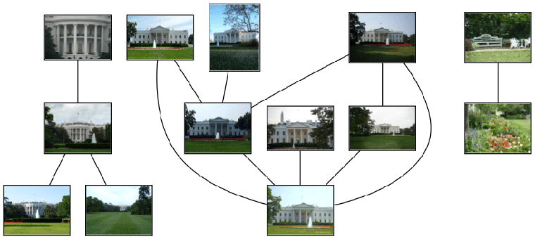 正如上图所示,我们可以看到三组图像,前两组是白宫不同的侧面图片。上面这个例子只是一个利用局部描述子进行匹配的很简单的例子,我们并没有对匹配进行核实,在后面两个章节中,我们便可以对其进行核实了。
from: http://yongyuan.name/pcvwithpython/chapter2.html
Python计算机视觉:第二章 图像局部描述符相关推荐
- 图像特征提取——韦伯局部描述符(WLD)
一.原理及概述 韦伯局部描述符(WLD)是一种鲁棒性好.简单高效的局部特征描述符.WLD由两个部分组成:差分激励和梯度方向. 其具体算法是对于给定的一幅图像,通过对每个像素进行这两个分量的计算来提取其 ...
- 【操作系统】第二章--进程的描述与控制--笔记与理解(2)
笔记理解之后可以进行深入解释→[操作系统]第二章–进程的描述与控制–深入与解释(2) 文章目录 第二章--进程的描述与控制--笔记与理解(2) 经典进程的同步问题 生产者-消费者问题 读者-写者问题 ...
- Java代码韦伯分布_第十五节、韦伯局部描述符(WLD,附源码)
纹理作为一种重要的视觉线索,是图像中普遍存在而又难以描述的特征,图像的纹理特征一般是指图像上地物重复排列造成的灰度值有规则的分布.纹理特征的关键在于纹理特征的提取方法.目前,用于纹理特征提取的方法有很 ...
- 老卫带你学---WLD韦伯局部描述符
WLD韦伯局部描述符也是一种可以衡量图像纹理信息的特征. 在大多的据不描述符中,Gabor小波和LBP是常见的两种.本文将主要介绍另外一种纹理的描述算子WLD(Weber's Local Descri ...
- 17.5.8 韦伯局部描述符(Weber's Local Descriptor)
在大多的据不描述符中,Gabor小波和LBP是常见的两种.本文将主要介绍另外一种纹理的描述算子WLD(Weber's Local Descriptor),主要由两部分组成:差励(differentia ...
- 模拟进程创建、终止、阻塞、唤醒原语_操作系统第二章--进程的描述与控制
操作系统第二章--进程的描述与控制 前趋图和程序执行 前趋图 前趋图是一个有向无循环图DAG,用来描述进程之间执行的前后关系 初始结点:没有前趋的结点 终止结点:没有后继的结点 重量:表示该结点所含有 ...
- 【操作系统】 第二章 进程的描述与控制
第二章 进程的描述与控制 2.1 什么是进程 程序代码+相关数据+程序控制块PCB 当处理器开始执行一个程序的代码时,称这个执行的实体为进程 2.1.1 进程和进程控制块PCB PCB(Process ...
- 操作系统 第二章 进程的描述与控制(4)进程同步(重点)
计算机操作系统 读书笔记 第二章 进程的描述与控制 进程同步(重点) 计算机操作系统 前言 进程同步 一.进程同步的基本概念 1.1 两种形式的制约关系 1.2 临界资源(Critical Resou ...
- 操作系统第二章进程的描述与控制
第二章进程的描述与控制 前驱图和程序执行 程序并发执行 程序的并发执行 程序并发执行时的特征 间断性 失去封闭性 不可再现性 进程的描述 进程的定义 进程是程序的一次执行 进程是一个程序及其数据在处理 ...
最新文章
- linux cpu %us,Linux top里面%CPU和us%的解释
- 如何实现可以获取最小值的栈?
- Bugku—MISC题总结
- AppBoxFuture(四). 随需而变-Online Schema Change
- [数据结构-严蔚敏版]P61ADT Queue的表示与实现(单链队列-队列的链式存储结构)
- 椒盐噪声加噪的实现原理
- 【NOIP2001】【Luogu1049】装箱问题
- shell 判断目录还是文件
- Java 定时器 Timer 与 定时任务 TimeTask
- HDU 1596 find the safest road
- 极限编程的12个实践原则
- 安卓手机抓包方法归纳总结
- 留言板php添加图片_php实现留言板功能
- php使用halt中断输出
- Doris开启Stream Load记录
- 机器人中的yaw/pitch/roll
- 面向对象基础案例(2)
- DDR4 硬件设计笔记
- 热电阻与热电偶的区别
- 照片位置信息提取(获取经纬度)