NetCDF4文件处理

• 下载MACA v2的 netcdf4 格式数据
• 使用 xarray 读取和处理 netcdf4 格式数据
• 将 netcdf4 格式数据导出为 .csv 格式
• 将 netcdf4 格式数据导出为 .tif 格式

参考链接

import osimport numpy as np
import pandas as pd
import matplotlib.pyplot as plt
# 处理netcdf4文件所要用到的包
import xarray as xr
import rioxarray
import cartopy.crs as ccrs
import cartopy.feature as cfeature
import seaborn as sns
import geopandas as gpd
import earthpy as et# 统计图绘制选项
sns.set(font_scale=1.3)
sns.set_style("white")

文件读取

.nc文件名的含义

agg_macav2metdata_tasmax_BNU-ESM_r1i1p1_historical_1950_2005_CONUS_monthly

• agg_macav2metdata ：MACA v2版本，降尺度到美国大陆
• tasmax ：数据项为最高温度
• BNU-ESM ：产生该原始数据的模式名称
• historical ：数据为1950-2005年的历史预测数据
• CONUS ：数据范围为美国（CONtinental United States boundary）
• monthly ：数据的时间分辨率为月份

# MACAv2数据连接
data_path = "http://thredds.northwestknowledge.net:8080/thredds/dodsC/agg_macav2metdata_tasmax_BNU-ESM_r1i1p1_historical_1950_2005_CONUS_monthly.nc"# 打开数据
with xr.open_dataset(data_path) as file_nc:# 使用 rio.write _ crs，确保数据的坐标系在整个分析过程中都保持不变max_temp_xr = file_nc.rio.write_crs(file_nc.rio.crs, inplace=True)# 查看数据对象
max_temp_xr

# 读取数据的坐标系统信息
climate_crs = max_temp_xr.rio.crs
climate_crs

CRS.from_wkt('GEOGCS["undefined",DATUM["undefined",SPHEROID["undefined",6378137,298.257223563]],PRIMEM["undefined",0],UNIT["degree",0.0174532925199433,AUTHORITY["EPSG","9122"]],AXIS["Longitude",EAST],AXIS["Latitude",NORTH]]')

# 查看前五行数据max_temp_xr['air_temperature']['lat'].values[:5]# 输出经纬度的最大值和最小值
print("The min and max latitude values in the data is:", max_temp_xr["air_temperature"]["lat"].values.min(), max_temp_xr["air_temperature"]["lat"].values.max())
print("The min and max longitude values in the data is:", max_temp_xr["air_temperature"]["lon"].values.min(), max_temp_xr["air_temperature"]["lon"].values.max())

The min and max latitude values in the data is: 25.063077926635742 49.39602279663086
The min and max longitude values in the data is: 235.22784423828125 292.93524169921875

# 查看数据的时间范围
print("The earliest date in the data is:", max_temp_xr["air_temperature"]["time"].values.min())
print("The latest date in the data is:", max_temp_xr["air_temperature"]["time"].values.max())

The earliest date in the data is: 1950-01-15 00:00:00
The latest date in the data is: 2005-12-15 00:00:00

# 查看数据记录的总条数，本数据集共672条，即672个月
max_temp_xr["air_temperature"]["time"].values.shape

(672,)

# 查看数据的坐标系统信息
max_temp_xr["crs"]

# 查看数据的元数据
metadata = max_temp_xr.attrs
metadata

{'description': 'Multivariate Adaptive Constructed Analogs (MACA) method, version 2.3,Dec 2013.','id': 'MACAv2-METDATA','naming_authority': 'edu.uidaho.reacch','Metadata_Conventions': 'Unidata Dataset Discovery v1.0','Metadata_Link': '','cdm_data_type': 'FLOAT','title': 'Monthly aggregation of downscaled daily meteorological data of Monthly Average of Daily Maximum Near-Surface Air Temperature from College of Global Change and Earth System Science, Beijing Normal University (BNU-ESM) using the run r1i1p1 of the historical scenario.','summary': 'This archive contains monthly downscaled meteorological and hydrological projections for the Conterminous United States at 1/24-deg resolution. These monthly values are obtained by aggregating the daily values obtained from the downscaling using the Multivariate Adaptive Constructed Analogs (MACA, Abatzoglou, 2012) statistical downscaling method with the METDATA (Abatzoglou,2013) training dataset. The downscaled meteorological variables are maximum/minimum temperature(tasmax/tasmin), maximum/minimum relative humidity (rhsmax/rhsmin),precipitation amount(pr), downward shortwave solar radiation(rsds), eastward wind(uas), northward wind(vas), and specific humidity(huss). The downscaling is based on the 365-day model outputs from different global climate models (GCMs) from Phase 5 of the Coupled Model Inter-comparison Project (CMIP3) utlizing the historical (1950-2005) and future RCP4.5/8.5(2006-2099) scenarios. ','keywords': 'monthly, precipitation, maximum temperature, minimum temperature, downward shortwave solar radiation, specific humidity, wind velocity, CMIP5, Gridded Meteorological Data','keywords_vocabulary': '','standard_name_vocabulary': 'CF-1.0','history': 'No revisions.','comment': '','geospatial_bounds': 'POLYGON((-124.7722 25.0631,-124.7722 49.3960, -67.0648 49.3960,-67.0648, 25.0631, -124.7722,25.0631))','geospatial_lat_min': '25.0631','geospatial_lat_max': '49.3960','geospatial_lon_min': '-124.7722','geospatial_lon_max': '-67.0648','geospatial_lat_units': 'decimal degrees north','geospatial_lon_units': 'decimal degrees east','geospatial_lat_resolution': '0.0417','geospatial_lon_resolution': '0.0417','geospatial_vertical_min': 0.0,'geospatial_vertical_max': 0.0,'geospatial_vertical_resolution': 0.0,'geospatial_vertical_positive': 'up','time_coverage_start': '2000-01-01T00:0','time_coverage_end': '2004-12-31T00:00','time_coverage_duration': 'P5Y','time_coverage_resolution': 'P1M','date_created': '2014-05-15','date_modified': '2014-05-15','date_issued': '2014-05-15','creator_name': 'John Abatzoglou','creator_url': 'http://maca.northwestknowledge.net','creator_email': 'jabatzoglou@uidaho.edu','institution': 'University of Idaho','processing_level': 'GRID','project': '','contributor_name': 'Katherine C. Hegewisch','contributor_role': 'Postdoctoral Fellow','publisher_name': 'REACCH','publisher_email': 'reacch@uidaho.edu','publisher_url': 'http://www.reacchpna.org/','license': 'Creative Commons CC0 1.0 Universal Dedication(http://creativecommons.org/publicdomain/zero/1.0/legalcode)','coordinate_system': 'WGS84,EPSG:4326','grid_mapping': 'crs'}

# 可以以调用字典的方式，查看元数据中的数据项目
# 如查看数据标题
metadata["title"]

'Monthly aggregation of downscaled daily meteorological data of Monthly Average of Daily Maximum Near-Surface Air Temperature from College of Global Change and Earth System Science, Beijing Normal University (BNU-ESM) using the run r1i1p1 of the historical scenario.'

在xarray数据中，使用 .sel() 方法可以快速提取数据子集

# 根据经纬度进行取值
key=400
longitude = max_temp_xr["air_temperature"]["lon"].values[key]
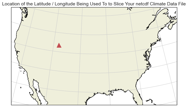
latitude = max_temp_xr["air_temperature"]["lat"].values[key]print("Long, Lat values:", longitude, latitude)

Long, Lat values: 251.89422607421875 41.72947692871094

在地图上显示选取点的位置

extent = [-120, -70, 24, 50.5]
central_lon = np.mean(extent[:2])
central_lat = np.mean(extent[2:])f, ax = plt.subplots(figsize=(12, 6),subplot_kw={'projection': ccrs.AlbersEqualArea(central_lon, central_lat)})
ax.coastlines()
# Plot the selected location
ax.plot(longitude-360, latitude, '^', transform=ccrs.PlateCarree(),color="r", markersize=15)ax.set_extent(extent)
ax.set(title="Location of the Latitude / Longitude Being Used To to Slice Your netcdf Climate Data File")# Adds continent boundaries to the map
ax.add_feature(cfeature.LAND, edgecolor='black')ax.gridlines()
plt.show()

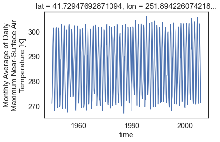
# 使用.sel()方法提取对应经纬度位置的数据
one_point=max_temp_xr["air_temperature"].sel(lat=latitude,lon=longitude)one_point

# 提取具体点位置的数据结果为该点的时间序列数据
one_point.shape

(672,)

# 查看该点上的前五条数据
one_point.values[:5]

array([271.11615, 274.05585, 279.538  , 284.42365, 294.1337 ],dtype=float32)

# 直接使用xarray直接绘制该点数据的时间序列折线图
one_point.plot()
plt.show()

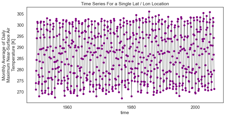
# 使用matplotlib绘制统计图
f, ax = plt.subplots(figsize=(12, 6))
one_point.plot.line(hue='lat',marker="o",ax=ax,color="grey",markerfacecolor="purple",markeredgecolor="purple")
ax.set(title="Time Series For a Single Lat / Lon Location")# 导出为png格式
# plt.savefig("single_point_timeseries.png")
plt.show()

将 xarray 数据转换成 Pandas DataFrame 格式并导出为 csv 文件

# 转换为DataFrame
one_point_df = one_point.to_dataframe()
# View just the first 5 rows of the data
one_point_df.head()

# pd导出为.csv文件
one_point_df.to_csv("one-location.csv")

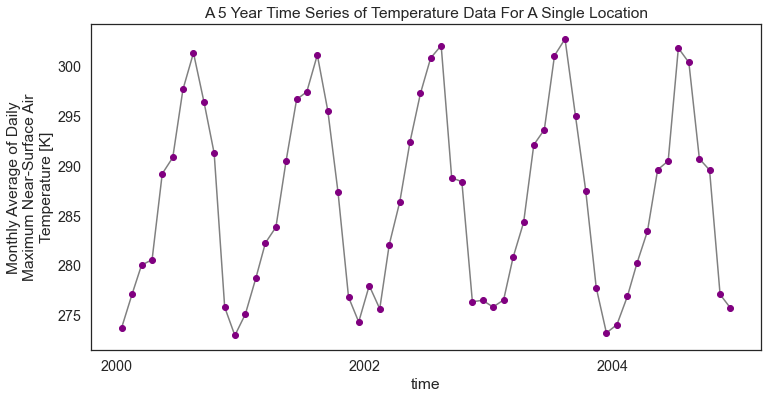
根据时间和地点对数据进行切片

start_date="2000-01-01"
end_date="2005-01-01"temp_2000_2005=max_temp_xr['air_temperature'].sel(time=slice(start_date,end_date),lat=45.02109146118164,lon=243.01937866210938)
temp_2000_2005

查看切片得到的数据信息

temp_2000_2005.shape

(60,)

切片时间段内的时间序列数据显示

# Plot the data just like you did above
f, ax = plt.subplots(figsize=(12, 6))
temp_2000_2005.plot.line(hue='lat',marker="o",ax=ax,color="grey",markerfacecolor="purple",markeredgecolor="purple")
ax.set(title="A 5 Year Time Series of Temperature Data For A Single Location")
plt.show()

对特定时间段以及指定的空间范围内的数据进行切片

# 设定起始和结束时间
start_date = "1950-01-15"
end_date = "1950-02-15"two_months_conus = max_temp_xr["air_temperature"].sel(time=slice(start_date, end_date))
# 查看切片后的数据信息
two_months_conus.shape

(2, 585, 1386)

# two_months_conus.plot()
# plt.show()

数据的空间可视化

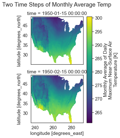
# 使用xarray.plot()可以对数据进行快速可视化
two_months_conus.plot(x="lon",y="lat",col="time", # 属性值col_wrap=1) # 按列绘制
plt.suptitle("Two Time Steps of Monthly Average Temp", y=1.03)
plt.show()

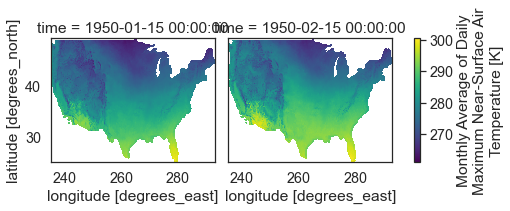
two_months_conus.plot(x="lon",y="lat",col="time",col_wrap=2)# 按行绘制
plt.show()

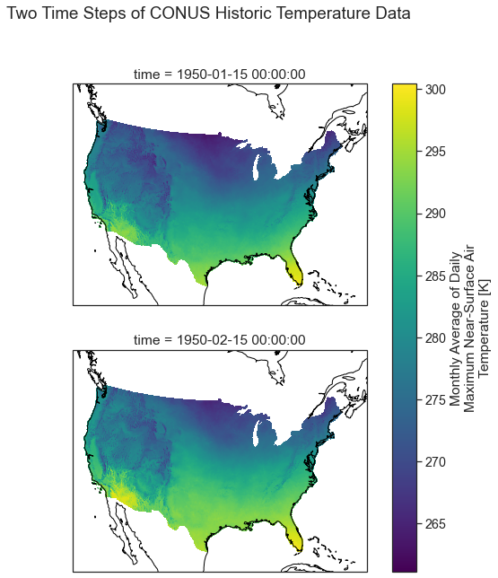
# 使用matplotlib绘制地图
central_lat = 37.5
central_long = 96
extent = [-120, -70, 20, 55.5]  # CONUSmap_proj = ccrs.AlbersEqualArea(central_longitude=central_lon,central_latitude=central_lat)aspect = two_months_conus.shape[2] / two_months_conus.shape[1]
p = two_months_conus.plot(transform=ccrs.PlateCarree(),  # the data's projectioncol='time', col_wrap=1,aspect=aspect,figsize=(10, 10),subplot_kws={'projection': map_proj})  # the plot's projectionplt.suptitle("Two Time Steps of CONUS Historic Temperature Data", y=1)
# Add the coastlines to each axis object and set extent
for ax in p.axes.flat:ax.coastlines()ax.set_extent(extent)

d:\ProgramData\Anaconda3\envs\pygis\lib\site-packages\xarray\plot\facetgrid.py:373: UserWarning: Tight layout not applied. The left and right margins cannot be made large enough to accommodate all axes decorations. self.fig.tight_layout()

将数据导出为Geotiff文件

• 使用 rioxarray 将数据导出为 geotiff文件格式

# 确保导出的数据带有坐标信息
two_months_conus.rio.crs

CRS.from_wkt('GEOGCS["undefined",DATUM["undefined",SPHEROID["undefined",6378137,298.257223563]],PRIMEM["undefined",0],UNIT["degree",0.0174532925199433,AUTHORITY["EPSG","9122"]],AXIS["Longitude",EAST],AXIS["Latitude",NORTH]]')

# 导出为tif文件
file_path = "two_months_temp_data.tif"
two_months_conus.rio.to_raster(file_path)

# 读取导出的tif文件
two_months_tiff = xr.open_rasterio(file_path)
two_months_tiff

# 查看数据的波段信息
two_months_tiff.plot()
plt.show()

# 绘制数据
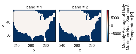
two_months_tiff.plot(col="band")
plt.show()

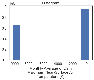
two_months_tiff.rio.nodata

-9999.0

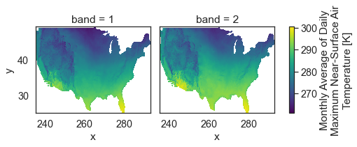
# 使用.where() to mask函数进行掩膜
two_months_tiff = xr.open_rasterio(file_path)two_months_clean = two_months_tiff.where(two_months_tiff != two_months_tiff.rio.nodata)two_months_clean.plot(col="band")
plt.show()

文章代码：

https://gitee.com/jiangroubao/learning/blob/master/NetCDF4/