SSD( Single Shot MultiBox Detector)关键源码解析
1,多尺度特征图检测网络结构;
2,anchor boxes生成;
3,ground truth预处理;
4,目标函数;
5,总结
<img src="https://pic2.zhimg.com/v2-d0252b7d1408105470b88ceb45054725_b.png" data-rawwidth="1031" data-rawheight="686" class="origin_image zh-lightbox-thumb" width="1031" data-original="https://pic2.zhimg.com/v2-d0252b7d1408105470b88ceb45054725_r.png">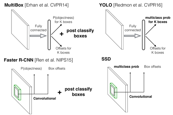
图0-1 SSD与MultiBox,Faster R-CNN,YOLO原理(此图来源于作者在eccv2016的PPT)
<img src="https://pic2.zhimg.com/v2-0213e22e8b0d96f8854e82d796c83a71_b.png" class="content_image">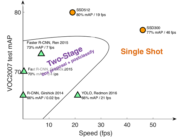
图0-2 SSD检测速度与精确度。(此图来源于作者在eccv2016的PPT)
1 多尺度特征图检测网络结构
SSD的网络模型如图1-1所示。<img src="https://pic1.zhimg.com/v2-7f7f3c99d20df97455e8bcfce7876d30_b.png" data-rawwidth="1152" data-rawheight="553" class="origin_image zh-lightbox-thumb" width="1152" data-original="https://pic1.zhimg.com/v2-7f7f3c99d20df97455e8bcfce7876d30_r.png">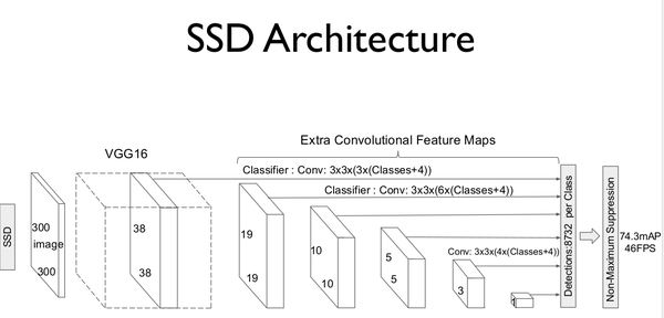
图1-1 SSD模型结构。(此图来源于原论文)
模型建立源代码包含于ssd_vgg_300.py中。模型多尺度特征图检测如图1-2所示。模型选择的特征图包括:38×38(block4),19×19(block7),10×10(block8),5×5(block9),3×3(block10),1×1(block11)。对于每张特征图,生成采用3×3卷积生成 默认框的四个偏移位置和21个类别的置信度。比如block7,默认框(def boxes)数目为6,每个默认框包含4个偏移位置和21个类别置信度(4+21)。因此,block7的最后输出为(19*19)*6*(4+21)。
<img src="https://pic1.zhimg.com/v2-5964f6dff6dbbd435336cde9e5dfc988_b.png" class="content_image">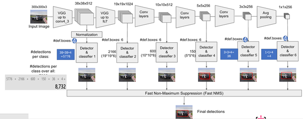
图1-2 多尺度特征采样(此图来源:知乎专栏)
其中,初始化参数如下:
    """
    Implementation of the SSD VGG-based 300 network.    The default features layers with 300x300 image input are:
      conv4 ==> 38 x 38
      conv7 ==> 19 x 19
      conv8 ==> 10 x 10
      conv9 ==> 5 x 5
      conv10 ==> 3 x 3
      conv11 ==> 1 x 1
    The default image size used to train this network is 300x300.
    """default_params = SSDParams(img_shape=(300, 300),#输入尺寸num_classes=21,#预测类别20+1=21(20类加背景)#获取feature map层feat_layers=['block4', 'block7', 'block8', 'block9', 'block10', 'block11'],feat_shapes=[(38, 38), (19, 19), (10, 10), (5, 5), (3, 3), (1, 1)],anchor_size_bounds=[0.15, 0.90],#anchor boxes的大小anchor_sizes=[(21., 45.),(45., 99.),(99., 153.),(153., 207.),(207., 261.),(261., 315.)],#anchor boxes的aspect ratiosanchor_ratios=[[2, .5],[2, .5, 3, 1./3],[2, .5, 3, 1./3],[2, .5, 3, 1./3],[2, .5],[2, .5]],anchor_steps=[8, 16, 32, 64, 100, 300],#anchor的层anchor_offset=0.5,#补偿阀值0.5normalizations=[20, -1, -1, -1, -1, -1],#该特征层是否正则,大于零即正则;小于零则否prior_scaling=[0.1, 0.1, 0.2, 0.2])
建立模型代码如下,作者采用了TensorFlow-Slim(类似于keras的高层库)来建立网络模型,详细内容可以参考TensorFlow-Slim网页。
#建立ssd网络函数
def ssd_net(inputs,num_classes=21,feat_layers=SSDNet.default_params.feat_layers,anchor_sizes=SSDNet.default_params.anchor_sizes,anchor_ratios=SSDNet.default_params.anchor_ratios,normalizations=SSDNet.default_params.normalizations,is_training=True,dropout_keep_prob=0.5,prediction_fn=slim.softmax,reuse=None,scope='ssd_300_vgg'):"""SSD net definition.
    """# End_points collect relevant activations for external use.#用于收集每一层输出结果end_points = {}#采用slim建立vgg网络,网络结构参考文章内的结构图with tf.variable_scope(scope, 'ssd_300_vgg', [inputs], reuse=reuse):# Original VGG-16 blocks.net = slim.repeat(inputs, 2, slim.conv2d, 64, [3, 3], scope='conv1')end_points['block1'] = netnet = slim.max_pool2d(net, [2, 2], scope='pool1')# Block 2.net = slim.repeat(net, 2, slim.conv2d, 128, [3, 3], scope='conv2')end_points['block2'] = netnet = slim.max_pool2d(net, [2, 2], scope='pool2')# Block 3.net = slim.repeat(net, 3, slim.conv2d, 256, [3, 3], scope='conv3')end_points['block3'] = netnet = slim.max_pool2d(net, [2, 2], scope='pool3')# Block 4.net = slim.repeat(net, 3, slim.conv2d, 512, [3, 3], scope='conv4')end_points['block4'] = netnet = slim.max_pool2d(net, [2, 2], scope='pool4')# Block 5.net = slim.repeat(net, 3, slim.conv2d, 512, [3, 3], scope='conv5')end_points['block5'] = netnet = slim.max_pool2d(net, [3, 3], 1, scope='pool5')#max pool#外加的SSD层# Additional SSD blocks.# Block 6: let's dilate the hell out of it!#输出shape为19×19×1024net = slim.conv2d(net, 1024, [3, 3], rate=6, scope='conv6')end_points['block6'] = net# Block 7: 1x1 conv. Because the fuck.#卷积核为1×1net = slim.conv2d(net, 1024, [1, 1], scope='conv7')end_points['block7'] = net# Block 8/9/10/11: 1x1 and 3x3 convolutions stride 2 (except lasts).end_point = 'block8'with tf.variable_scope(end_point):net = slim.conv2d(net, 256, [1, 1], scope='conv1x1')net = slim.conv2d(net, 512, [3, 3], stride=2, scope='conv3x3')end_points[end_point] = netend_point = 'block9'with tf.variable_scope(end_point):net = slim.conv2d(net, 128, [1, 1], scope='conv1x1')net = slim.conv2d(net, 256, [3, 3], stride=2, scope='conv3x3')end_points[end_point] = netend_point = 'block10'with tf.variable_scope(end_point):net = slim.conv2d(net, 128, [1, 1], scope='conv1x1')net = slim.conv2d(net, 256, [3, 3], scope='conv3x3', padding='VALID')end_points[end_point] = netend_point = 'block11'with tf.variable_scope(end_point):net = slim.conv2d(net, 128, [1, 1], scope='conv1x1')net = slim.conv2d(net, 256, [3, 3], scope='conv3x3', padding='VALID')end_points[end_point] = net# Prediction and localisations layers.#预测和定位predictions = []logits = []localisations = []for i, layer in enumerate(feat_layers):with tf.variable_scope(layer + '_box'):#接受特征层的输出,生成类别和位置预测p, l = ssd_multibox_layer(end_points[layer],num_classes,anchor_sizes[i],anchor_ratios[i],normalizations[i])#把每一层的预测收集predictions.append(prediction_fn(p))#prediction_fn为softmax,预测类别logits.append(p)#概率localisations.append(l)#预测位置信息return predictions, localisations, logits, end_points
2 anchor box生成
对每一张特征图,按照不同的大小(scale) 和长宽比(ratio) 生成生成k个默认框(default boxes),原理图如图2-1所示(此图中,默认框数目k=6,其中5×5的红色点代表特征图,因此:5*5*6 = 150 个boxes)。
每个默认框大小计算公式为:,其中,m为特征图数目,
为最底层特征图大小(原论文中值为0.2,代码中为0.15),
为最顶层特征图默认框大小(原论文中为0.9,代码中为0.9)。
每个默认框长宽比根据比例值计算,原论文中比例值为,因此,每个默认框的宽为
,高为
。对于比例为1的默认框,额外添加一个比例为
的默认框。最终,每张特征图中的每个点生成6个默认框。每个默认框中心设定为
,其中,
为第k个特征图尺寸。
<img src="https://pic4.zhimg.com/v2-e128c01e26456fa24502e2c05bf46e1b_b.png" class="content_image"><img src="https://pic3.zhimg.com/v2-e6f0dd799661fff724853435b976a82e_b.png" class="content_image"><img src="https://pic3.zhimg.com/v2-64a521f37e62fe79c9b5d11746eb6686_b.png" class="content_image">
图2-1 anchor box生成示意图(此图来源于知乎专栏)
源代码中,默认框生成函数为ssd_anchor_one_layer(),代码如下:
#生成一层的anchor boxes
def ssd_anchor_one_layer(img_shape,#原始图像shapefeat_shape,#特征图shapesizes,#预设的box sizeratios,#aspect 比例step,#anchor的层offset=0.5,dtype=np.float32):"""Computer SSD default anchor boxes for one feature layer.    Determine the relative position grid of the centers, and the relative
    width and height.    Arguments:
      feat_shape: Feature shape, used for computing relative position grids;
      size: Absolute reference sizes;
      ratios: Ratios to use on these features;
      img_shape: Image shape, used for computing height, width relatively to the
        former;
      offset: Grid offset.    Return:
      y, x, h, w: Relative x and y grids, and height and width.
    """# Compute the position grid: simple way.# y, x = np.mgrid[0:feat_shape[0], 0:feat_shape[1]]# y = (y.astype(dtype) + offset) / feat_shape[0]# x = (x.astype(dtype) + offset) / feat_shape[1]# Weird SSD-Caffe computation using steps values..."""
    #测试中,参数如下
    feat_shapes=[(38, 38), (19, 19), (10, 10), (5, 5), (3, 3), (1, 1)]
    anchor_sizes=[(21., 45.),
                      (45., 99.),
                      (99., 153.),
                      (153., 207.),
                      (207., 261.),
                      (261., 315.)]
    anchor_ratios=[[2, .5],
                       [2, .5, 3, 1./3],
                       [2, .5, 3, 1./3],
                       [2, .5, 3, 1./3],
                       [2, .5],
                       [2, .5]]
    anchor_steps=[8, 16, 32, 64, 100, 300]    offset=0.5    dtype=np.float32    feat_shape=feat_shapes[0]
    step=anchor_steps[0]
    """#测试中,y和x的shape为(38,38)(38,38)#y的值为#array([[ 0,  0,  0, ...,  0,  0,  0],#  [ 1,  1,  1, ...,  1,  1,  1],# [ 2,  2,  2, ...,  2,  2,  2],#   ..., #  [35, 35, 35, ..., 35, 35, 35],#  [36, 36, 36, ..., 36, 36, 36],#  [37, 37, 37, ..., 37, 37, 37]])y, x = np.mgrid[0:feat_shape[0], 0:feat_shape[1]]#测试中y=(y+0.5)×8/300,x=(x+0.5)×8/300y = (y.astype(dtype) + offset) * step / img_shape[0]x = (x.astype(dtype) + offset) * step / img_shape[1]#扩展维度,维度为(38,38,1)# Expand dims to support easy broadcasting.y = np.expand_dims(y, axis=-1)x = np.expand_dims(x, axis=-1)# Compute relative height and width.# Tries to follow the original implementation of SSD for the order.#数值为2+2num_anchors = len(sizes) + len(ratios)#shape为(4,)h = np.zeros((num_anchors, ), dtype=dtype)w = np.zeros((num_anchors, ), dtype=dtype)# Add first anchor boxes with ratio=1.#测试中,h[0]=21/300,w[0]=21/300?h[0] = sizes[0] / img_shape[0]w[0] = sizes[0] / img_shape[1]di = 1if len(sizes) > 1:#h[1]=sqrt(21*45)/300h[1] = math.sqrt(sizes[0] * sizes[1]) / img_shape[0]w[1] = math.sqrt(sizes[0] * sizes[1]) / img_shape[1]di += 1for i, r in enumerate(ratios):h[i+di] = sizes[0] / img_shape[0] / math.sqrt(r)w[i+di] = sizes[0] / img_shape[1] * math.sqrt(r)#测试中,y和x shape为(38,38,1)#h和w的shape为(4,)return y, x, h, w
3 ground truth预处理
训练过程中,首先需要将label信息(ground truth box,ground truth category)进行预处理,将其对应到相应的默认框上。根据默认框和ground truth box的jaccard 重叠来寻找对应的默认框。文章中选取了jaccard重叠超过0.5的默认框为正样本,其它为负样本。
源代码ground truth预处理代码位于ssd_common.py文件中,关键代码如下:
#label和bbox编码函数
def tf_ssd_bboxes_encode_layer(labels,#ground truth标签,1D tensorbboxes,#N×4 Tensor(float)anchors_layer,#anchors,为listmatching_threshold=0.5,#阀值prior_scaling=[0.1, 0.1, 0.2, 0.2],#缩放dtype=tf.float32):"""Encode groundtruth labels and bounding boxes using SSD anchors from
    one layer.    Arguments:
      labels: 1D Tensor(int64) containing groundtruth labels;
      bboxes: Nx4 Tensor(float) with bboxes relative coordinates;
      anchors_layer: Numpy array with layer anchors;
      matching_threshold: Threshold for positive match with groundtruth bboxes;
      prior_scaling: Scaling of encoded coordinates.    Return:
      (target_labels, target_localizations, target_scores): Target Tensors.
    """# Anchors coordinates and volume.#获取anchors层yref, xref, href, wref = anchors_layerymin = yref - href / 2.xmin = xref - wref / 2.ymax = yref + href / 2.xmax = xref + wref / 2.#xmax的shape为((38, 38, 1), (38, 38, 1), (4,), (4,))
(38, 38, 4)#体积vol_anchors = (xmax - xmin) * (ymax - ymin)# Initialize tensors...shape = (yref.shape[0], yref.shape[1], href.size)feat_labels = tf.zeros(shape, dtype=tf.int64)feat_scores = tf.zeros(shape, dtype=dtype)#shape为(38,38,4)feat_ymin = tf.zeros(shape, dtype=dtype)feat_xmin = tf.zeros(shape, dtype=dtype)feat_ymax = tf.ones(shape, dtype=dtype)feat_xmax = tf.ones(shape, dtype=dtype)#计算jaccard重合def jaccard_with_anchors(bbox):"""Compute jaccard score a box and the anchors.
        """# Intersection bbox and volume.int_ymin = tf.maximum(ymin, bbox[0])int_xmin = tf.maximum(xmin, bbox[1])int_ymax = tf.minimum(ymax, bbox[2])int_xmax = tf.minimum(xmax, bbox[3])h = tf.maximum(int_ymax - int_ymin, 0.)w = tf.maximum(int_xmax - int_xmin, 0.)# Volumes.inter_vol = h * wunion_vol = vol_anchors - inter_vol \+ (bbox[2] - bbox[0]) * (bbox[3] - bbox[1])jaccard = tf.div(inter_vol, union_vol)return jaccard#条件函数 def condition(i, feat_labels, feat_scores,feat_ymin, feat_xmin, feat_ymax, feat_xmax):"""Condition: check label index.
        """#tf.less函数 Returns the truth value of (x < y) element-wise.r = tf.less(i, tf.shape(labels))return r[0]#主体def body(i, feat_labels, feat_scores,feat_ymin, feat_xmin, feat_ymax, feat_xmax):"""Body: update feature labels, scores and bboxes.
        Follow the original SSD paper for that purpose:
          - assign values when jaccard > 0.5;
          - only update if beat the score of other bboxes.
        """# Jaccard score.label = labels[i]bbox = bboxes[i]scores = jaccard_with_anchors(bbox)#计算jaccard重合值# 'Boolean' mask.#tf.greater函数返回大于的布尔值mask = tf.logical_and(tf.greater(scores, matching_threshold),tf.greater(scores, feat_scores))imask = tf.cast(mask, tf.int64)fmask = tf.cast(mask, dtype)# Update values using mask.feat_labels = imask * label + (1 - imask) * feat_labelsfeat_scores = tf.select(mask, scores, feat_scores)feat_ymin = fmask * bbox[0] + (1 - fmask) * feat_yminfeat_xmin = fmask * bbox[1] + (1 - fmask) * feat_xminfeat_ymax = fmask * bbox[2] + (1 - fmask) * feat_ymaxfeat_xmax = fmask * bbox[3] + (1 - fmask) * feat_xmaxreturn [i+1, feat_labels, feat_scores,feat_ymin, feat_xmin, feat_ymax, feat_xmax]# Main loop definition.i = 0[i, feat_labels, feat_scores,feat_ymin, feat_xmin,feat_ymax, feat_xmax] = tf.while_loop(condition, body,[i, feat_labels, feat_scores,feat_ymin, feat_xmin,feat_ymax, feat_xmax])# Transform to center / size.#计算补偿后的中心feat_cy = (feat_ymax + feat_ymin) / 2.feat_cx = (feat_xmax + feat_xmin) / 2.feat_h = feat_ymax - feat_yminfeat_w = feat_xmax - feat_xmin# Encode features.feat_cy = (feat_cy - yref) / href / prior_scaling[0]feat_cx = (feat_cx - xref) / wref / prior_scaling[1]feat_h = tf.log(feat_h / href) / prior_scaling[2]feat_w = tf.log(feat_w / wref) / prior_scaling[3]# Use SSD ordering: x / y / w / h instead of ours.feat_localizations = tf.stack([feat_cx, feat_cy, feat_w, feat_h], axis=-1)return feat_labels, feat_localizations, feat_scores#ground truth编码函数
def tf_ssd_bboxes_encode(labels,#ground truth标签,1D tensorbboxes,#N×4 Tensor(float)anchors,#anchors,为listmatching_threshold=0.5,#阀值prior_scaling=[0.1, 0.1, 0.2, 0.2],#缩放dtype=tf.float32,scope='ssd_bboxes_encode'):"""Encode groundtruth labels and bounding boxes using SSD net anchors.
    Encoding boxes for all feature layers.    Arguments:
      labels: 1D Tensor(int64) containing groundtruth labels;
      bboxes: Nx4 Tensor(float) with bboxes relative coordinates;
      anchors: List of Numpy array with layer anchors;
      matching_threshold: Threshold for positive match with groundtruth bboxes;
      prior_scaling: Scaling of encoded coordinates.    Return:
      (target_labels, target_localizations, target_scores):
        Each element is a list of target Tensors.
    """with tf.name_scope(scope):target_labels = []target_localizations = []target_scores = []for i, anchors_layer in enumerate(anchors):with tf.name_scope('bboxes_encode_block_%i' % i):#将label和bbox进行编码t_labels, t_loc, t_scores = \tf_ssd_bboxes_encode_layer(labels, bboxes, anchors_layer,matching_threshold, prior_scaling, dtype)target_labels.append(t_labels)target_localizations.append(t_loc)target_scores.append(t_scores)return target_labels, target_localizations, target_scores#编码goundtruth的label和bboxdef bboxes_encode(self, labels, bboxes, anchors,scope='ssd_bboxes_encode'):"""Encode labels and bounding boxes.
        """return ssd_common.tf_ssd_bboxes_encode(labels, bboxes, anchors,matching_threshold=0.5,prior_scaling=self.params.prior_scaling,scope=scope)
4 目标函数
SSD目标函数分为两个部分:对应默认框的位置loss(loc)和类别置信度loss(conf)。定义 为第i个默认框和对应的第j个ground truth box,相应的类别为p。目标函数定义为:
其中,N为匹配的默认框。如果N=0,loss为零。为预测框
和ground truth box
的Smooth L1 loss,
值通过cross validation设置为1。
<img src="https://pic2.zhimg.com/v2-f7f9cd187a7e4cf8fb2c430a844bdc5d_b.png" data-rawwidth="441" data-rawheight="93" class="origin_image zh-lightbox-thumb" width="441" data-original="https://pic2.zhimg.com/v2-f7f9cd187a7e4cf8fb2c430a844bdc5d_r.png">
定义如下:<img src="https://pic1.zhimg.com/v2-c59028fcd350680c60002216cac34434_b.png" data-rawwidth="539" data-rawheight="184" class="origin_image zh-lightbox-thumb" width="539" data-original="https://pic1.zhimg.com/v2-c59028fcd350680c60002216cac34434_r.png">其中,其中,
为预测框,
为ground truth。
为补偿(regress to offsets)后的默认框(
)的中心,
为默认框的宽和高。
定义为多累别softmax loss,公式如下:
<img src="https://pic3.zhimg.com/v2-b5772e77cfe447103133b90c05a807ee_b.png" data-rawwidth="739" data-rawheight="75" class="origin_image zh-lightbox-thumb" width="739" data-original="https://pic3.zhimg.com/v2-b5772e77cfe447103133b90c05a807ee_r.png">目标函数定义源码位于ssd_vgg_300.py,注释如下:
目标函数定义源码位于ssd_vgg_300.py,注释如下:
# =========================================================================== #
# SSD loss function.
# =========================================================================== #
def ssd_losses(logits, #预测类别localisations,#预测位置gclasses, #ground truth 类别glocalisations, #ground truth 位置gscores,#ground truth 分数match_threshold=0.5,negative_ratio=3.,alpha=1.,label_smoothing=0.,scope='ssd_losses'):"""Loss functions for training the SSD 300 VGG network.    This function defines the different loss components of the SSD, and
    adds them to the TF loss collection.    Arguments:
      logits: (list of) predictions logits Tensors;
      localisations: (list of) localisations Tensors;
      gclasses: (list of) groundtruth labels Tensors;
      glocalisations: (list of) groundtruth localisations Tensors;
      gscores: (list of) groundtruth score Tensors;
    """# Some debugging...# for i in range(len(gclasses)):#     print(localisations[i].get_shape())#     print(logits[i].get_shape())#     print(gclasses[i].get_shape())#     print(glocalisations[i].get_shape())#     print()with tf.name_scope(scope):l_cross = []l_loc = []for i in range(len(logits)):with tf.name_scope('block_%i' % i):# Determine weights Tensor.pmask = tf.cast(gclasses[i] > 0, logits[i].dtype)n_positives = tf.reduce_sum(pmask)#正样本数目#np.prod函数Return the product of array elements over a given axisn_entries = np.prod(gclasses[i].get_shape().as_list())# r_positive = n_positives / n_entries# Select some random negative entries.r_negative = negative_ratio * n_positives / (n_entries - n_positives)#负样本数nmask = tf.random_uniform(gclasses[i].get_shape(),dtype=logits[i].dtype)nmask = nmask * (1. - pmask)nmask = tf.cast(nmask > 1. - r_negative, logits[i].dtype)#cross_entropy loss# Add cross-entropy loss.with tf.name_scope('cross_entropy'):# Weights Tensor: positive mask + random negative.weights = pmask + nmaskloss = tf.nn.sparse_softmax_cross_entropy_with_logits(logits[i],gclasses[i])loss = tf.contrib.losses.compute_weighted_loss(loss, weights)l_cross.append(loss)#smooth loss# Add localization loss: smooth L1, L2, ...with tf.name_scope('localization'):# Weights Tensor: positive mask + random negative.weights = alpha * pmaskloss = custom_layers.abs_smooth(localisations[i] - glocalisations[i])loss = tf.contrib.losses.compute_weighted_loss(loss, weights)l_loc.append(loss)# Total losses in summaries...with tf.name_scope('total'):tf.summary.scalar('cross_entropy', tf.add_n(l_cross))tf.summary.scalar('localization', tf.add_n(l_loc))
5 总结
本文对SSD: Single Shot MultiBox Detector的tensorflow的关键源代码进行了解析。本文采用的源码来自于balancap/SSD-Tensorflow。源码作者写得非常详细,内容较多(其它还包括了图像预处理,多GPU并行训练等许多内容),因此只选取了关键代码进行解析。在看完论文后,再结合关键代码分析,结构就很清晰了。SSD代码实现的关键点为:1,多尺度特征图检测网络结构;2,anchor boxes生成;3,ground truth预处理;4,目标函数。SSD和YOLOv2类似,可以实现高准确率下的实时目标检测,是非常值得研究和改进的目标检测方法。
SSD( Single Shot MultiBox Detector)关键源码解析相关推荐
- 深度学习之 SSD(Single Shot MultiBox Detector)
目标检测近年来已经取得了很重要的进展,主流的算法主要分为两个类型: (1)two-stage方法,如R-CNN系算法,其主要思路是先通过启发式方法(selective search)或者CNN网络(R ...
- SSD: Single Shot MultiBox Detector
SSD: Single Shot MultiBox Detector 一.SSD主要思想 SSD是Single Shot MultiBox Detector的缩写,Single shot表明了SS ...
- SSD(Single shot multibox detector)目标检测模型架构和设计细节分析
先给出论文链接:SSD: Single Shot MultiBox Detector 本文将对SSD中一些难以理解的细节做仔细分析,包括了default box和ground truth的结合,def ...
- 目标检测方法简介:RPN(Region Proposal Network) and SSD(Single Shot MultiBox Detector)
原文引用:http://lufo.me/2016/10/detection/ 最近几年深度学习在计算机视觉领域取得了巨大的成功,而在目标检测这一计算机视觉的经典问题上直到去年(2015)才有了完全使用 ...
- 目标检测--SSD: Single Shot MultiBox Detector
SSD: Single Shot MultiBox Detector ECCV2016 https://github.com/weiliu89/caffe/tree/ssd 针对目标检测问题,本文取消 ...
- SSD论文阅读(Wei Liu——【ECCV2016】SSD Single Shot MultiBox Detector)
本文转载自: http://www.cnblogs.com/lillylin/p/6207292.html SSD论文阅读(Wei Liu--[ECCV2016]SSD Single Shot Mul ...
- ssd网络结构_封藏的SSD(Single Shot MultiBox Detector)笔记
关注oldpan博客,侃侃而谈人工智能深度酝酿优质原创文! 阅读本文需要xx分钟 ? 前言 本文用于记录学习SSD目标检测的过程,并且总结一些精华知识点. 为什么要学习SSD,是因为SSD和YOLO一 ...
- SSD: Single Shot MultiBox Detector 之再阅读
SSD: Single Shot MultiBox Detector SSD 一句话就是速度快,效果好! 第一版 8 Dec 2015,第二版是30 Mar 2016 主要改进是内容更加详实,实验更加 ...
- 目标检测 SSD: Single Shot MultiBox Detector - SSD在MMDetection中的实现
目标检测 SSD: Single Shot MultiBox Detector - SSD在MMDetection中的实现 flyfish 目标检测 SSD: Single Shot MultiBox ...
最新文章
- RabbitMQ 七种队列模式应用场景案例分析(通俗易懂)
- 下次诺贝尔奖会是他吗?肠道微生物组领域开创者Jeffrey Gordon
- Markdown中数学公式练习
- 毕业设计开题计算机进度安排表,关于2021届本科毕业设计选题情况及开题时间的通知...
- node.js跨域问题
- 【GitHub】GitHub 的 Pull Request 和 GitLab 的 Merge Request 有区别吗?
- app+java_App Store 上的“Java大全”
- asp.net中慎用static全局变量
- 8-2-Listener监听器
- 终极算法:机器学习和人工智能如何重塑世界笔记(转)
- 网站压力测试的几种方法
- 在CSDN写博客教程
- 高频电子线路_实验一:调谐放大器
- WMS 怎么搞定库内拣选与分拣?
- 统计字符串中的大小写字母个数
- python中的matplotlib用法
- 不想玩大数据的厨子都不是冒险家
- Ardunio开发实例-MAX30102脉搏血氧饱和度和心率监测传感器
- 【JAVA Core】精品面试题100道
- 求助应用Netlogo做交通出行方式选择仿真
热门文章
- idea代码可以编译但是爆红_推荐一款 IDEA 生成代码神器,写代码再也不用加班了...
- lwip协议栈在linux运行,LwIP协议栈在uCOS II下的实现
- micopython 18b20_[MicroPython]stm32f407控制DS18B20检测温度
- python猴子偷桃_Python实例100个(基于最新Python3.7版本)
- postgresql 查询序列_RazorSQL for Mac(数据库工具查询) v9.0.9
- 东电计算机考研大概分数,2019年各学院硕士研究生拟录取名单公示
- java如何画百分比圆环_canvas绘制百分比圆环进度条
- caffe不支持relu6_国产AI框架再进化!百度Paddle Lite发布:率先支持华为NPU在线编译,全新架构更多硬件支持...
- 语言建立一个学生籍贯管理簿_编写一个Excel自定义函数,身份证信息提取如探囊取物...
- arraylist线程安全吗_Java的线程安全、单例模式、JVM内存结构等知识梳理